Tools

• Filters LAS/LAZ
• Ground classification
• LAS/LAZ Insta 360 Coloring
• PRJ editor
• Viewing the point cloud
• Data archive GNSS
• Track trimming
• Merge track files
• Trim IMR (+GNSS)
• Trim IMR
• Coordinate converter(One coordinate)
• Coordinate Converter(Coordinates from file)
• Maps
• GNSS data converter
• RINEX merger
• Satellite filtering
• Calculating the focal length

Filters LAS/LAZ

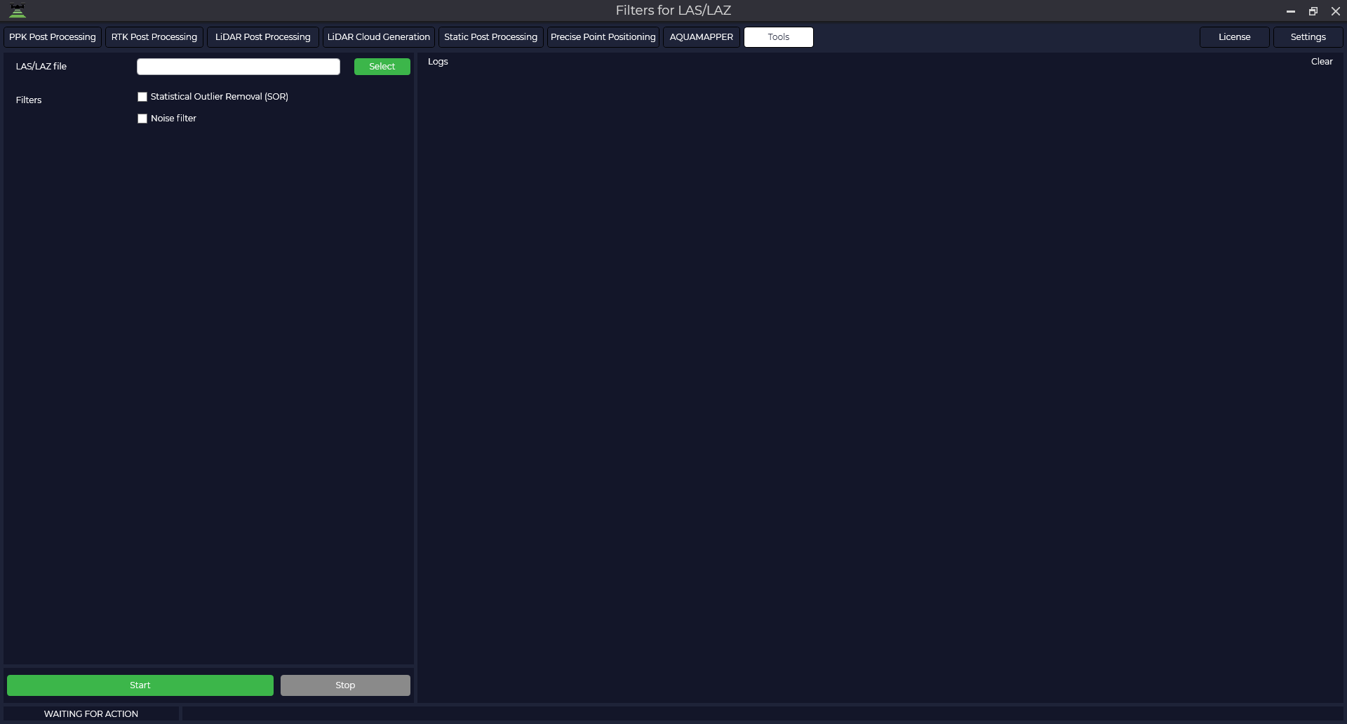
When launching the filters, we are greeted with a startup window.

Statistical Outlier Removal (SOR) is a method that first calculates the average distance between each point and its neighbors. It then removes points that are more than the average distance plus a few standard deviations. The minimum number of neighboring points is 6 and the standard deviation is 1.

Noise removal is a method that is similar to statistical outlier removal (SOR), but it considers the distance to the main surface rather than neighboring points. It locally fits a plane around each cloud point and removes a point if it is too far from that plane. This filter can be thought of as a low-point filter.

Surface reconstruction is a technique that is used to create complete surface models from heterogeneous data. Sometimes small errors in distance measurements can lead to difficulties in removing anomalies by statistical analysis. In such cases, surface reconstruction uses a resampling algorithm that attempts to reconstruct missing parts of the surface by polynomial interpolation between surrounding data points. This corrects small errors and smooths out artifacts such as "double walls" that occur when multiple scans are recorded simultaneously.

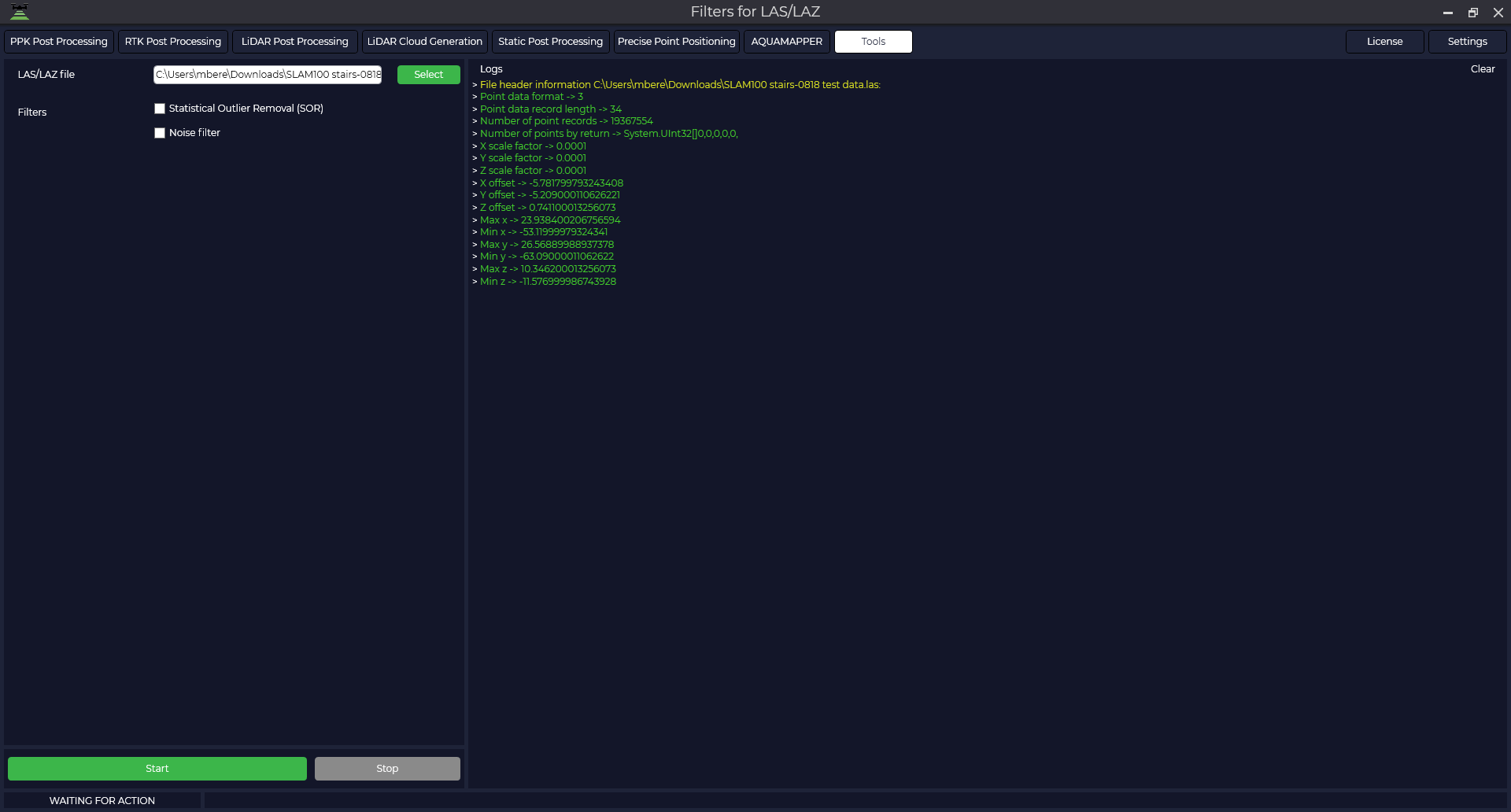
If you select a file in LAS or LAZ format, the login window will display the information contained in the file: number of points, X, Y, Z offsets, etc.

To process, check the required filters and press the "Start" button. If several filters are selected, they are applied sequentially. All results are saved to the folder with the source file.

Ground classification

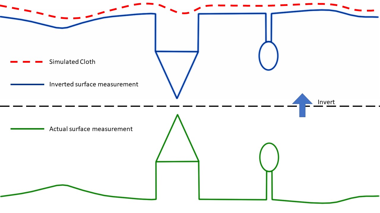
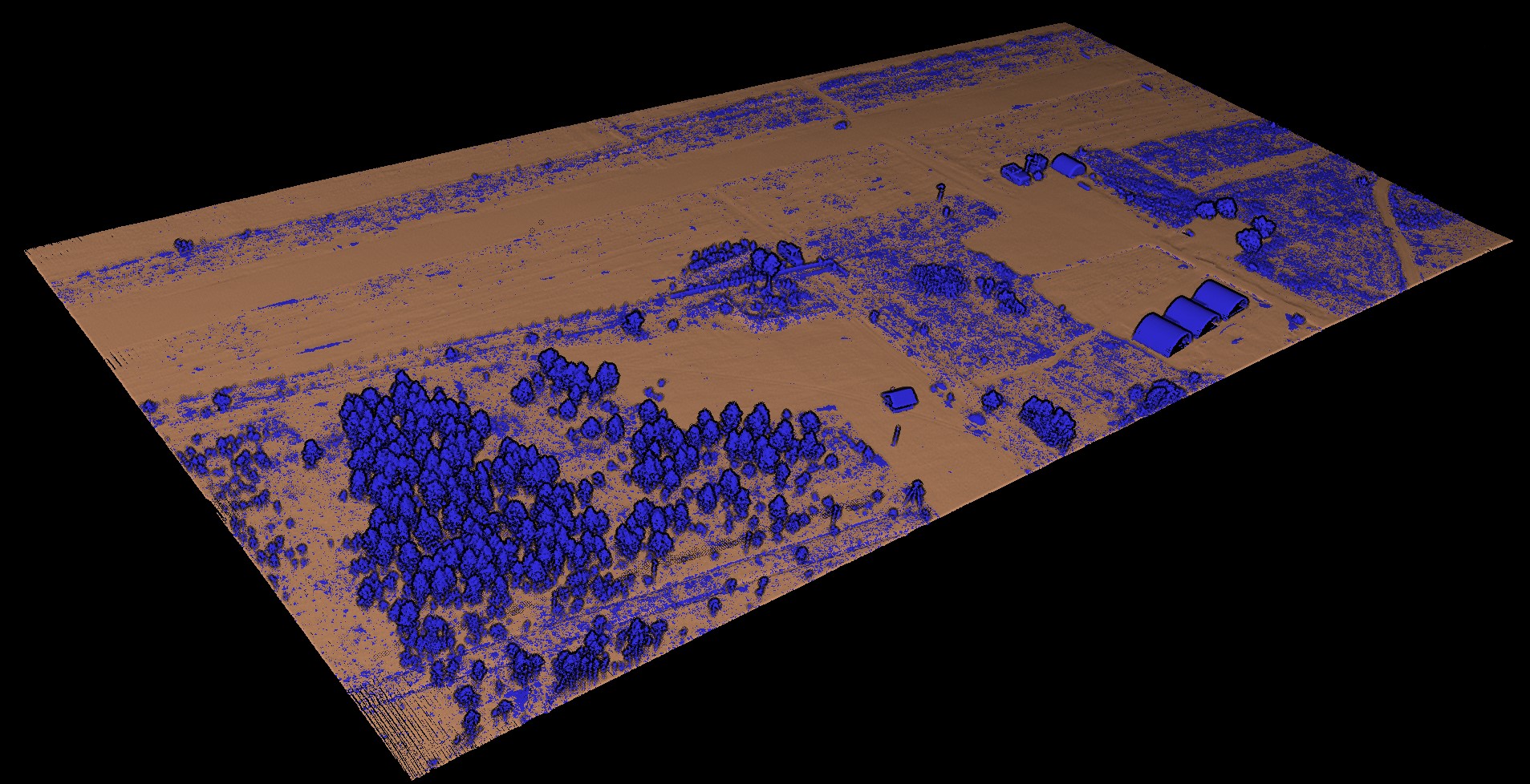
The Ground Classification tool allows you to divide the point cloud into two components: terrain related points and all other points. This method is based on a simplified physical process. Imagine a piece of cloth suspended above the terrain, which then falls down due to gravity. If the fabric is soft enough, it will stick to the surface and the final shape of the fabric will be a digital model of the terrain. However, if the point cloud is first turned upside down and the fabric is made stiff, the final shape will be a digital terrain model. A method called fabric modelling is used to model this process. Based on this method, a cloth modelling filtering (CSF) algorithm has been developed to extract ground points from the point cloud. An overview of the proposed algorithm is shown in Fig. First, the original point cloud is flipped upside down, and then a fabric is dropped on the flipped surface. By analysing the interaction between the fabric nodes and the corresponding points, the final shape of the fabric can be determined and used to classify the original points into terrain points and all other points.

When launching the tool, we are greeted with a startup window.

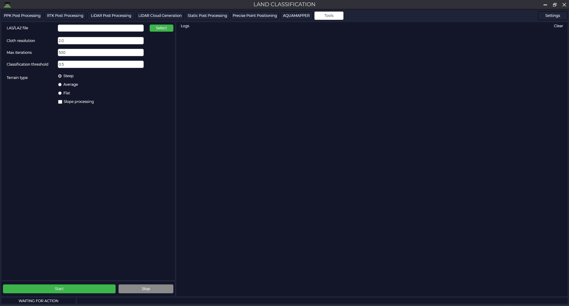
In the window that opens, click the "Select" button and select the file in the *.las or *.laz format for which you are going to make a classification. The Logs window displays information about the uploaded file.

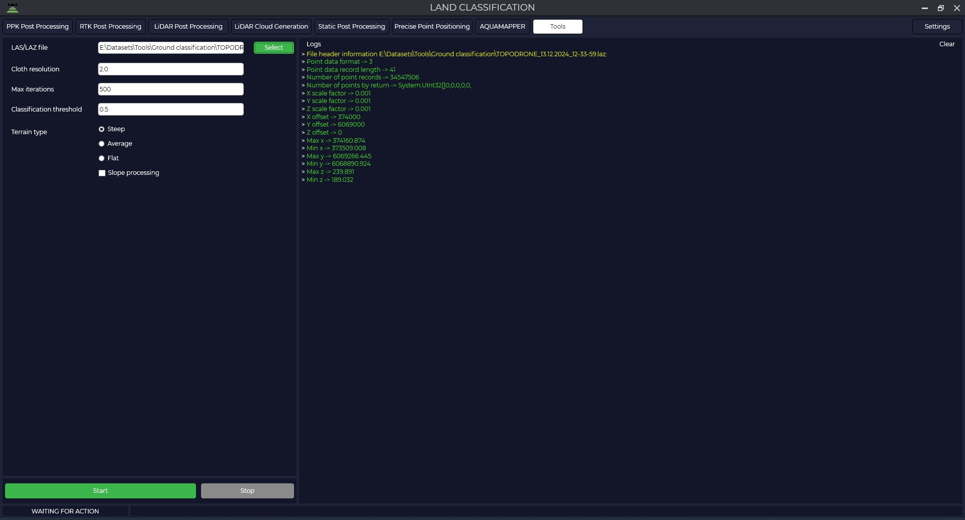
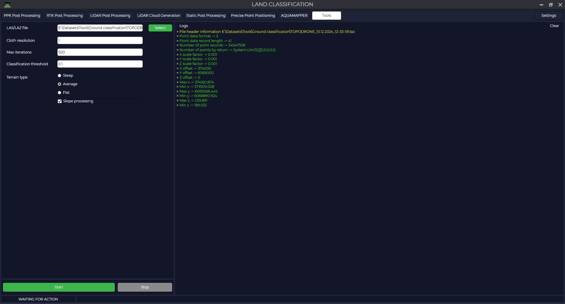
After that, set parameters that match the characteristics of your point cloud:
The grid step is the size of the grid cell, expressed in point cloud units, that is applied to cover the terrain. Increasing the grid resolution will result in a more detailed surface model, but will increase the computational load.
Number of iterations - the maximum allowable number of iterations performed during surface modelling. For most scenes it is recommended to set this value at 500 iterations, which is sufficient to achieve acceptable accuracy.
Classification tolerance - a parameter used to separate point clouds into ground related points and other points based on distances to the modelled terrain surface. The units of the tolerance must match the units of your point cloud. The recommended value for this parameter is 0.5, which is appropriate for most processing scenarios.
Terrain Type - with this parameter you can set the type of point cloud scene.

For steep slopes, this algorithm can produce relatively large errors because the modelled fabric is above the steep slopes and does not agree well with ground-based measurements due to internal constraints between particles.

Slope handling — the problem described above can be solved by selecting this option. If your scenes don't have steep slopes, just ignore it.

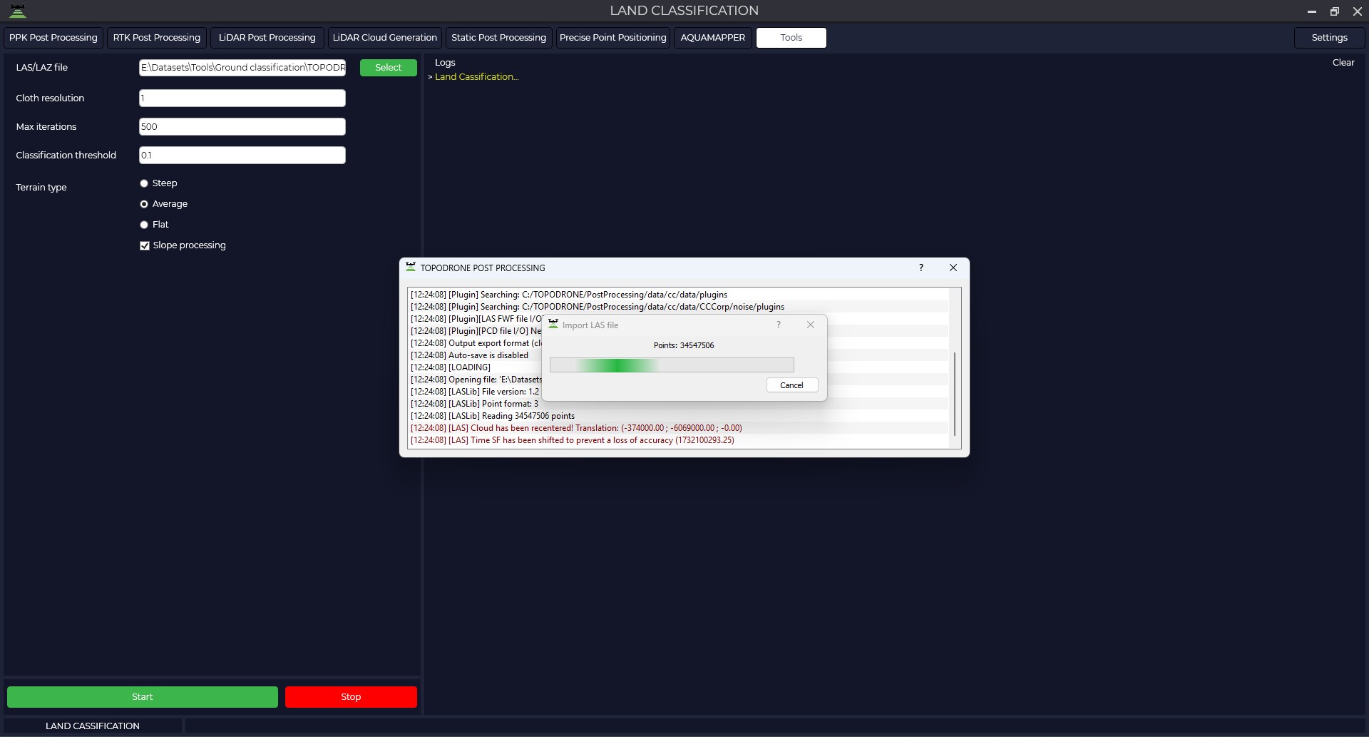
Press the ‘Start’ button and wait for the operation to complete.

The final result is the files: the ground point cloud and the rest of the points.

LAS/LAZ Insta 360 Coloring

This module is designed for automatically assigning color characteristics to a Mobile Laser Scanning (MLS) point cloud, coloring it with natural colors using data obtained from TOPODRONE scanning systems.

Operating Principle and Data Requirements:

To obtain a point cloud with reliable RGB information, the following processing sequence must be executed:

1. Primary Data Processing: Perform standard processing of raw data in the LiDAR Post Processing module to obtain the laser scanner's trajectory.

2. Point Cloud Generation: Generate the final point cloud in LAS/LAZ format using the LiDAR Cloud Generation module.

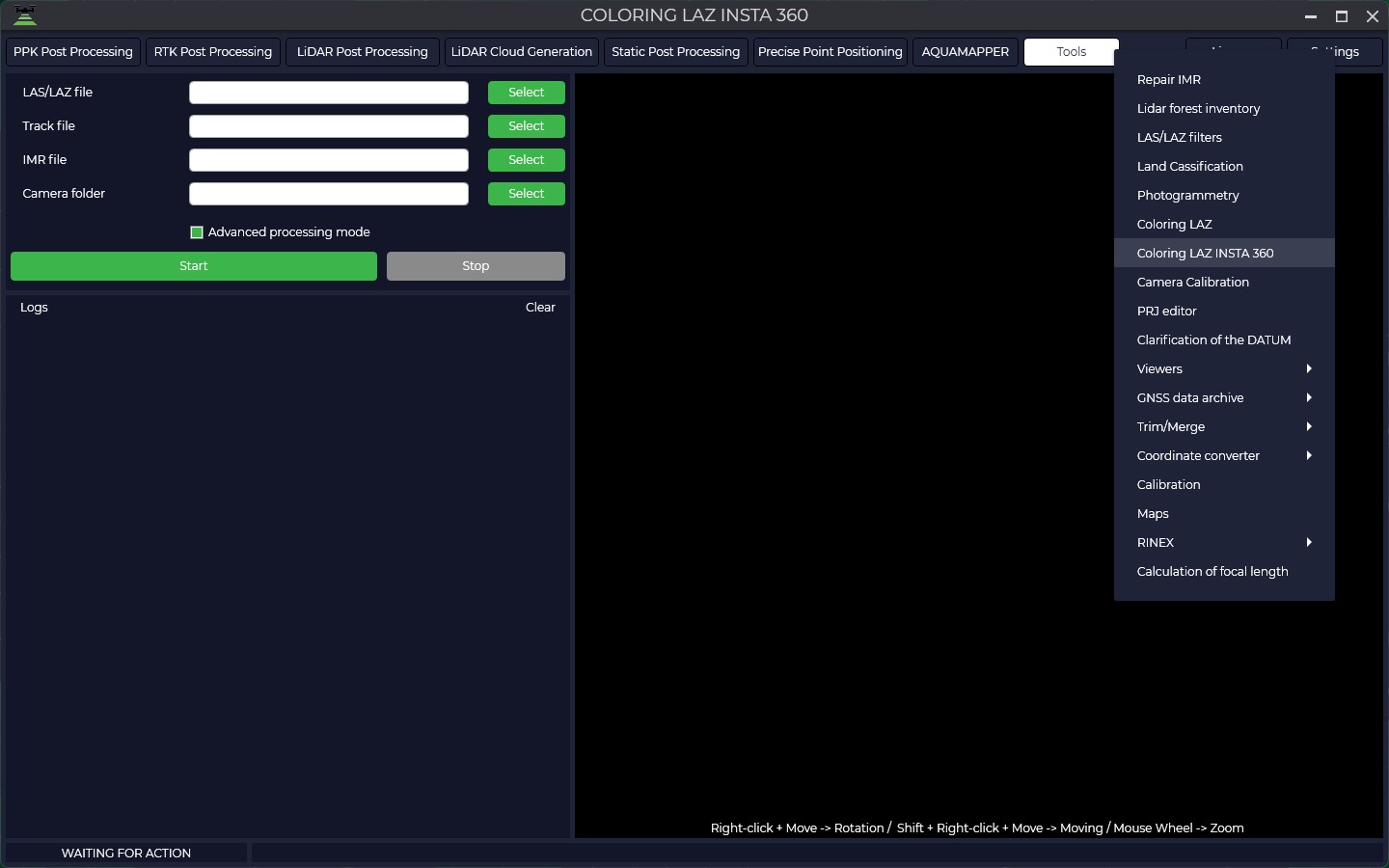
3. Point Cloud Coloring: At the final stage, using the "LAS/LAZ Insta 360 Coloring" tool, RGB values are assigned to the points in the cloud. The algorithm matches each laser reflection point with the corresponding pixel from the panoramic images taken by the Insta 360 camera, based on the precise trajectory and data about the camera's position relative to the laser scanner. This ensures realistic coloring in natural colors.

The point cloud coloring process involves several stages.

---

Data Preparation

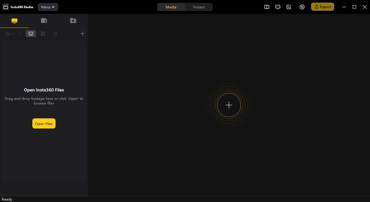
During recording, the Insta 360 camera saves data in its proprietary formats (*.lrv and *.insv). These formats are optimized for working with panoramic video in the manufacturer's software. For further processing, specifically for point cloud coloring, the video stream must be converted to the standard *.mp4 format. To do this, you need to install the Insta360 Studio program.

1. Launch the Insta360 Studio program.
   

   

   
   

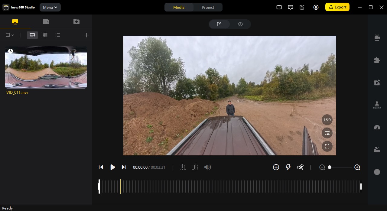
2. Import the source files (*.lrv and *.insv) into the project.
   

   

   
   

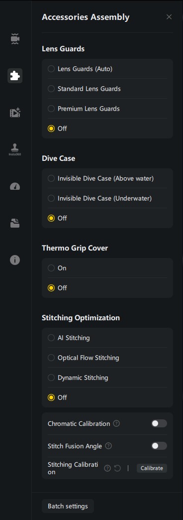
3. Navigate to the "Accessory Layout" tab and set the parameters according to the screenshot below.
   

   

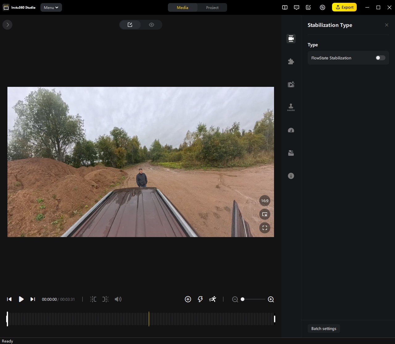
4. In the "Stabilization Type" tab, deactivate the "FlowState Stabilization" option by unchecking the corresponding box.
   

   

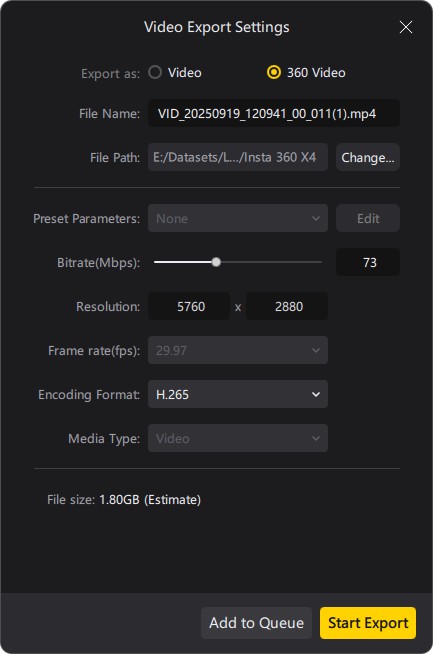
5. Initiate the export of the video file using the settings specified below into the folder containing the source *.lrv and *.insv files.
   

   

---

Point Cloud Coloring Process

Navigate to the "Tools" menu and select the "LAS/LAZ Insta 360 Coloring" module.

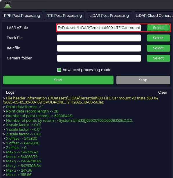
Specify the point cloud file in LAS/LAZ format, generated in the previous processing step in the "LiDAR Cloud Generation" module. This is an uncolored point cloud that contains spatial coordinates (X, Y, Z) and other laser information but lacks color attributes.

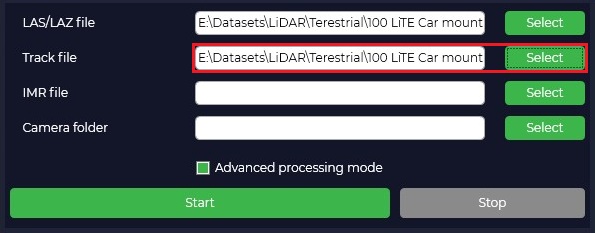
Select the trajectory file in the appropriate projection, obtained along with the point cloud from the "LiDAR Cloud Generation" module. The trajectory file contains precise coordinates and orientation of the scanning system at each moment in time. This data is critical for the temporal and spatial synchronization of frames with the cloud points.

Load the Inertial Measurement Unit (IMU) data file.

Specify the folder containing all the necessary video materials in *.lrv, *.insv, and *.mp4 formats.

 

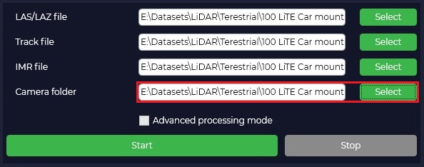
Click the "Start" button to initiate the coloring algorithm.
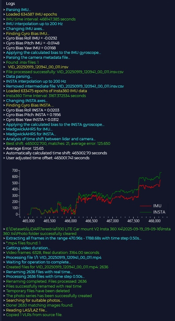
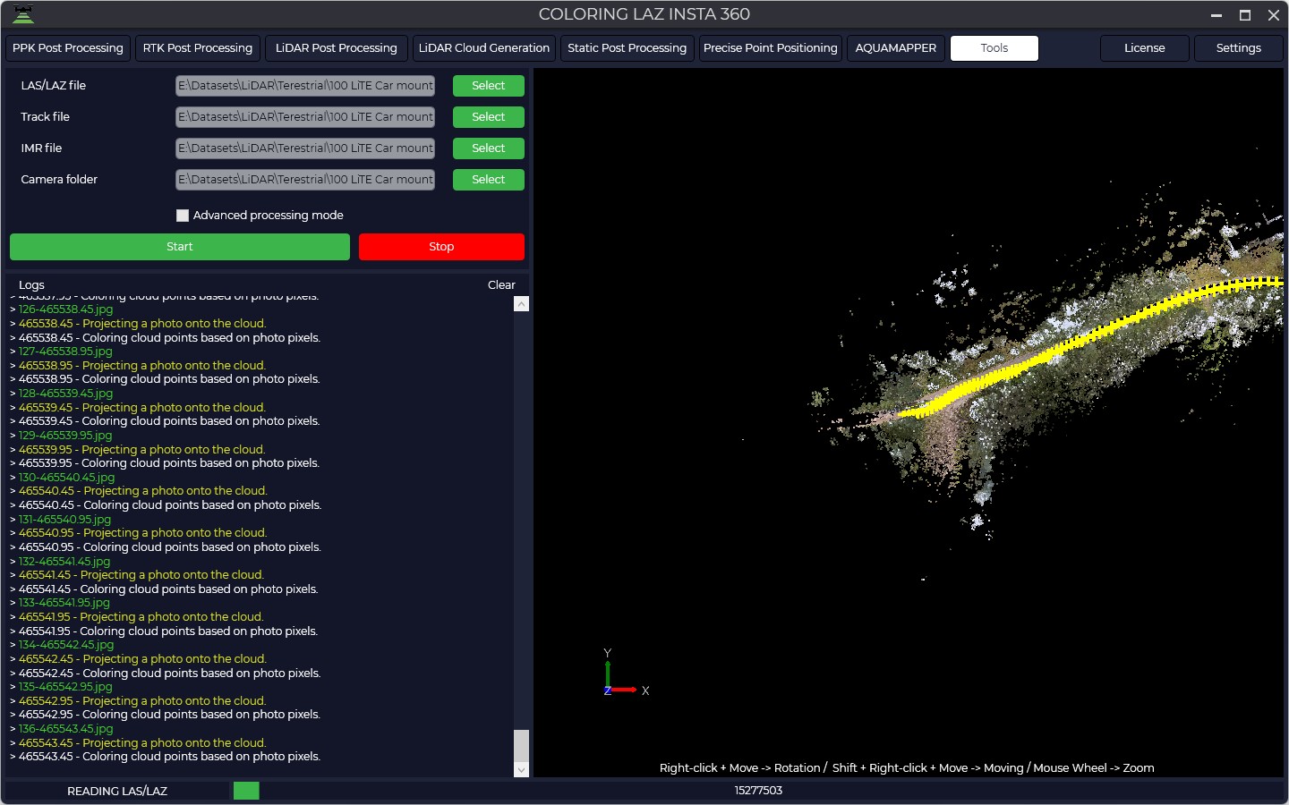
The processing progress is displayed in the "Log" text window. This window outputs information messages, warnings, and errors.

The "Viewer" window displays the process of assigning colors to the point cloud points in real-time, allowing for visual control over the processing accuracy.

Upon successful completion of the process, the module will automatically create a new file of the colored point cloud. The file is saved in the same directory as the source cloud. The prefix _RGB is added to the source filename for identification. A folder named "Photo" will be created in the directory containing the video files; this folder will contain panoramic images georeferenced to the WGS-84 coordinate system.

PRJ editor

PRJ Editor is a tool that allows you to edit the coordinate system knowing the transition parameters. In order to use it you need to select "PRJ Editor" in the Tools panel.

Currently, a small amount of photogrammetry and laser scanning software supports affine transformations, so this tool does not support affine transformations in the same way.

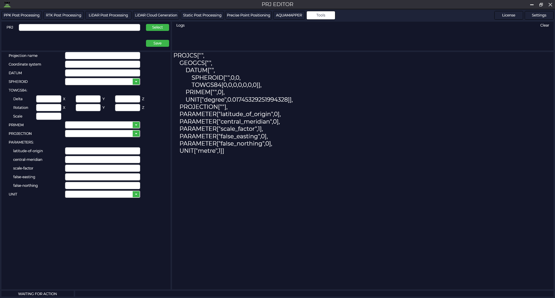
In the window that opens, click the "Select" button and select the *.prj file you want to edit.

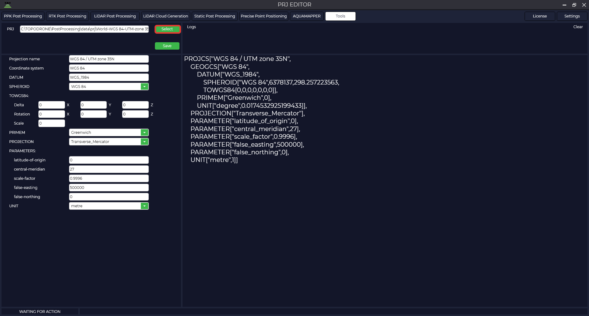
The table provides a description of the parameters

Projection name	WGS 84 / UTM zone 35N	Projection name
Coordinate system	WGS_1984	Name of coordinate system
DATUM	WGS_1984	Datum name
SPHEROID	WGS 84",6378137,298.257223563	Name of ellipsoid
TOWGS84		7 parameters of transition to WGS84
Delta	0,0,0	Displacement of the intermediate geocentric coordinate along the X, Y, Z axes. It is specified in meters, and the translation direction is indicated by the value sign.
Rotation	0,0,0	The amount of rotation about the X, Y, Z axes that applies to intermediate geocentric coordinates. It is specified in angular seconds, and the direction of translation is indicated by the sign of the value.
Scale	0	A scaling factor that applies to intermediate geocentric coordinates. The value is given in parts per million and is the difference between the actual scaling factor and one. For example, a scale parameter value of -2.5 gives an actual scale factor of 0.9999985. That is, the actual scale factor used is obtained by multiplying the parameter value by 1.0x10-06 and adding the result (algebraically) to 1.0.
PRIMEM	"Greenwich",0	Zero meridian, indicating the offset between the zero meridian of the declared coordinate system and the Greenwich coordinate system.
UNIT	"degree",0.01745329251994328	The unit of measure of SC (degrees).
PROJECTION	Transverse_Mercator	Projection type
PARAMETERS
Latitude of origin	0	Initial latitude
Central meridian	27	Central meridian
Scale factory	0.9996	Scale factor
False easting	500000	Shift east
False northing	0	Shift north
UNIT	metre	Projection unit

Make all necessary changes to the parameters, click the "Save" button, specify the path to save and the file name.

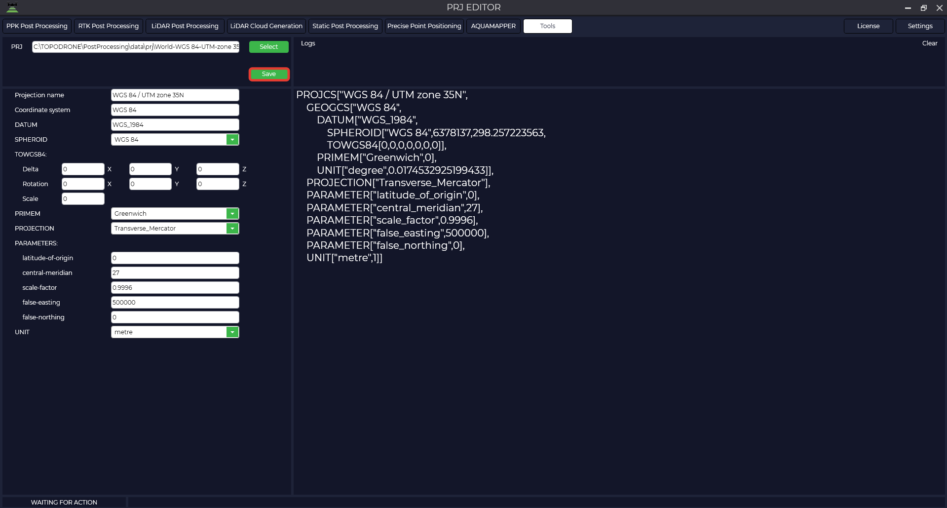
The resulting file is shown below.

PROJCS["WGS 84 / UTM zone 35N",
    GEOGCS["WGS 84",
        DATUM["WGS_1984",
            SPHEROID["WGS 84",6378137,298.257223563,
            TOWGS84[0,0,0,0,0,0,0]],
        PRIMEM["Greenwich",0,
        UNIT["degree",0.0174532925199433,
    PROJECTION["Transverse_Mercator"],
    PARAMETER["latitude_of_origin",0],
    PARAMETER["central_meridian",27],
    PARAMETER["scale_factor",0.9996],
    PARAMETER["false_easting",500000],
    PARAMETER["false_northing",0],
    UNIT["metre",1]]

Viewing the point cloud

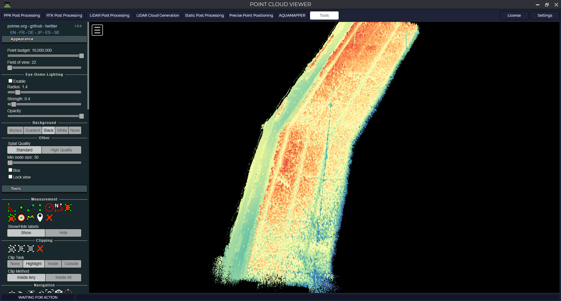
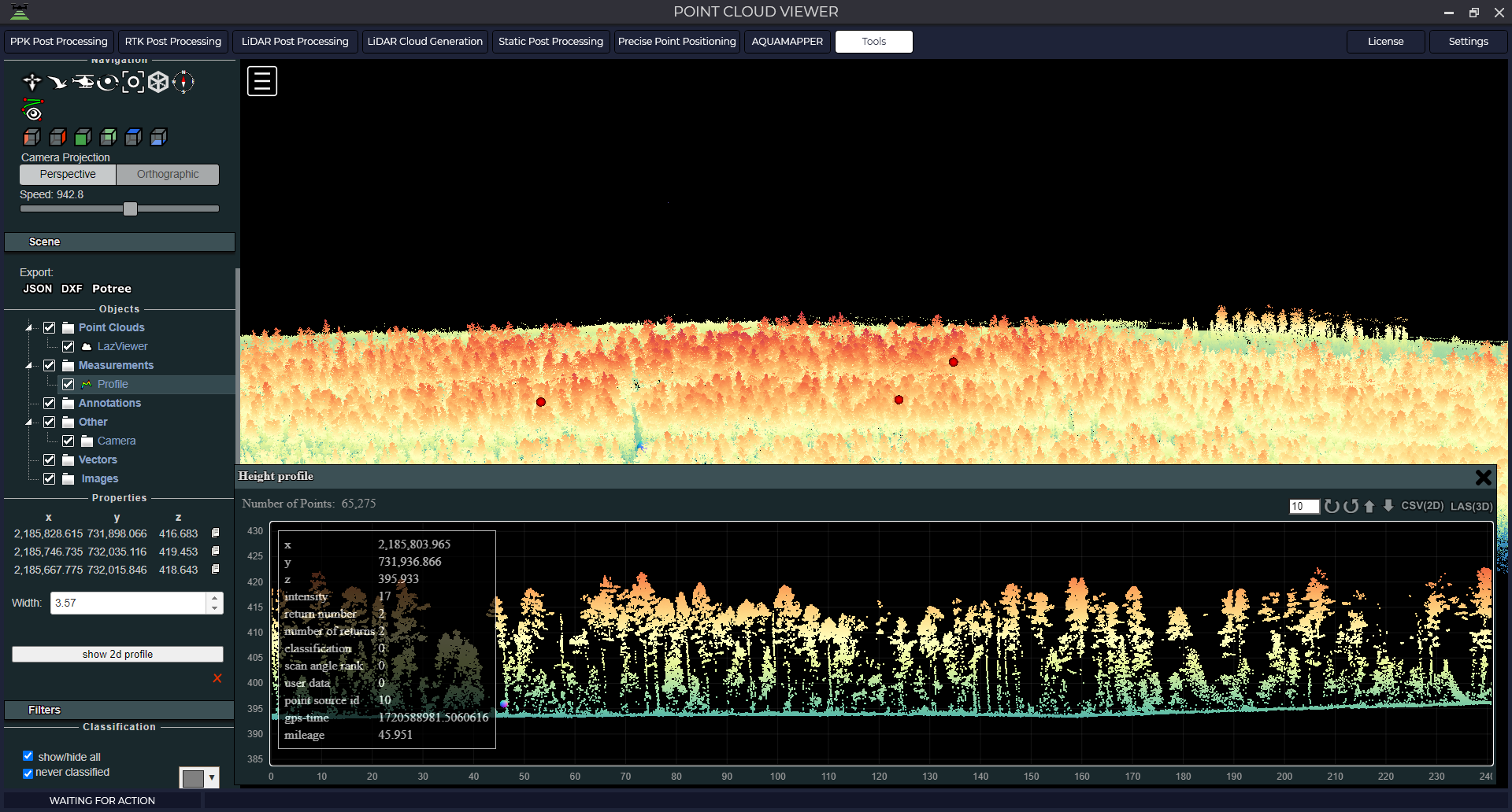
This tool is intended for viewing and analyzing the point cloud obtained during processing in TOPODRONE Post Processing software. To start the module, go to the Tools tab, then Viewers and click on the New button. If you need to open a point cloud that has just been closed, select Previous. In the opened tab select the point cloud in *.las or *.laz format. After loading, the point cloud will be displayed in the main window.

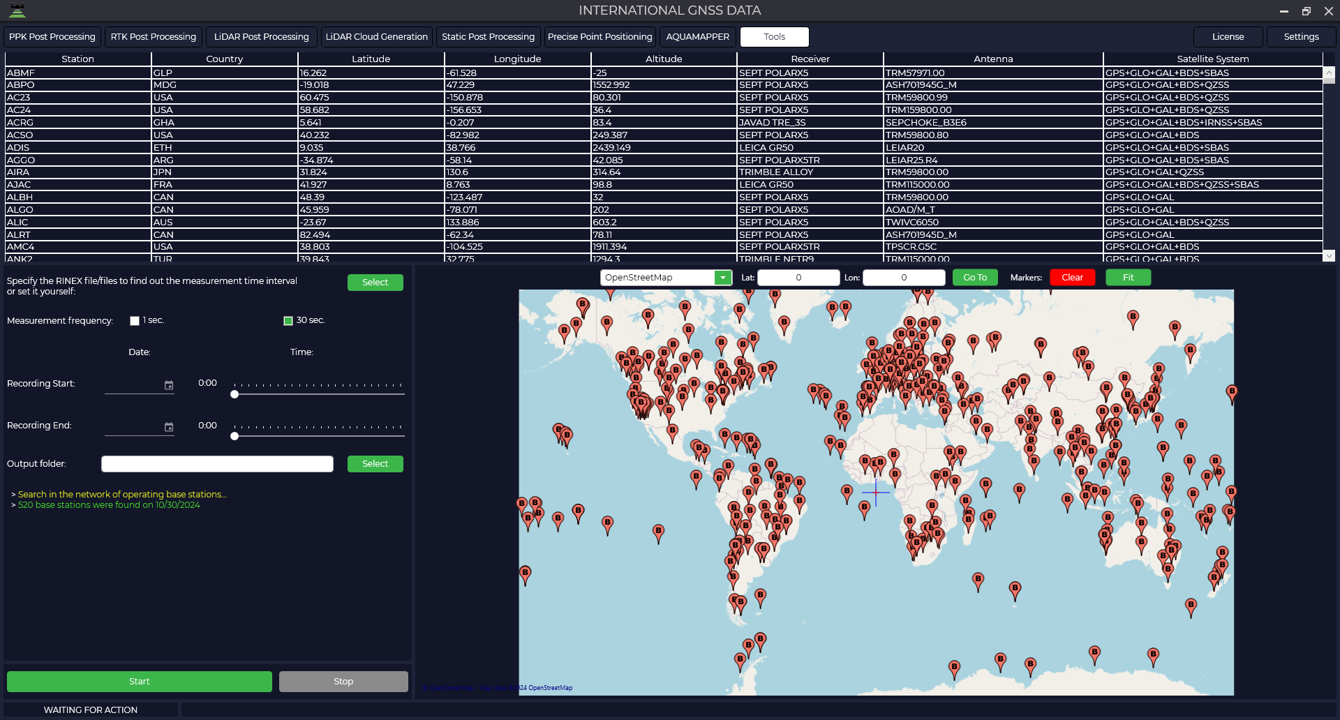
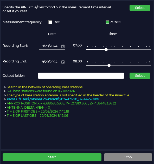
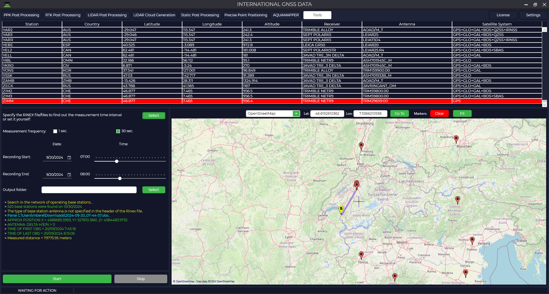
Data archive GNSS

This module is a large database with publicly available base stations for downloading observation files.

1. To start the module, go to the "Tools" tab, then "GNSS Data Archives" and select the database you need.
   

   

   
   
2. Then download the data from your receiver to have the program select the date and time of the base stations or enter this data manually. Specify the folder where you want to save the result.
   

   

3. In the table or on the map, select the base station from which you want to download data and press the "Start" button, the data download will start in the folder you specified.
   
   

   

   
   

Track trimming

This tool is designed to trim a trajectory file in *.pos and *.poses format.
To start the tool, select Track Trim in the Tools, Trim/Stitch tab. Then select the track you want to trim.

There are two sliders at the bottom, by moving them you specify the interval of the trajectory, which will remain and which will be cut. You will see a visual representation of the two colors on the trajectory. Green indicates the area that will be saved after trimming, and red indicates the area that will be trimmed.

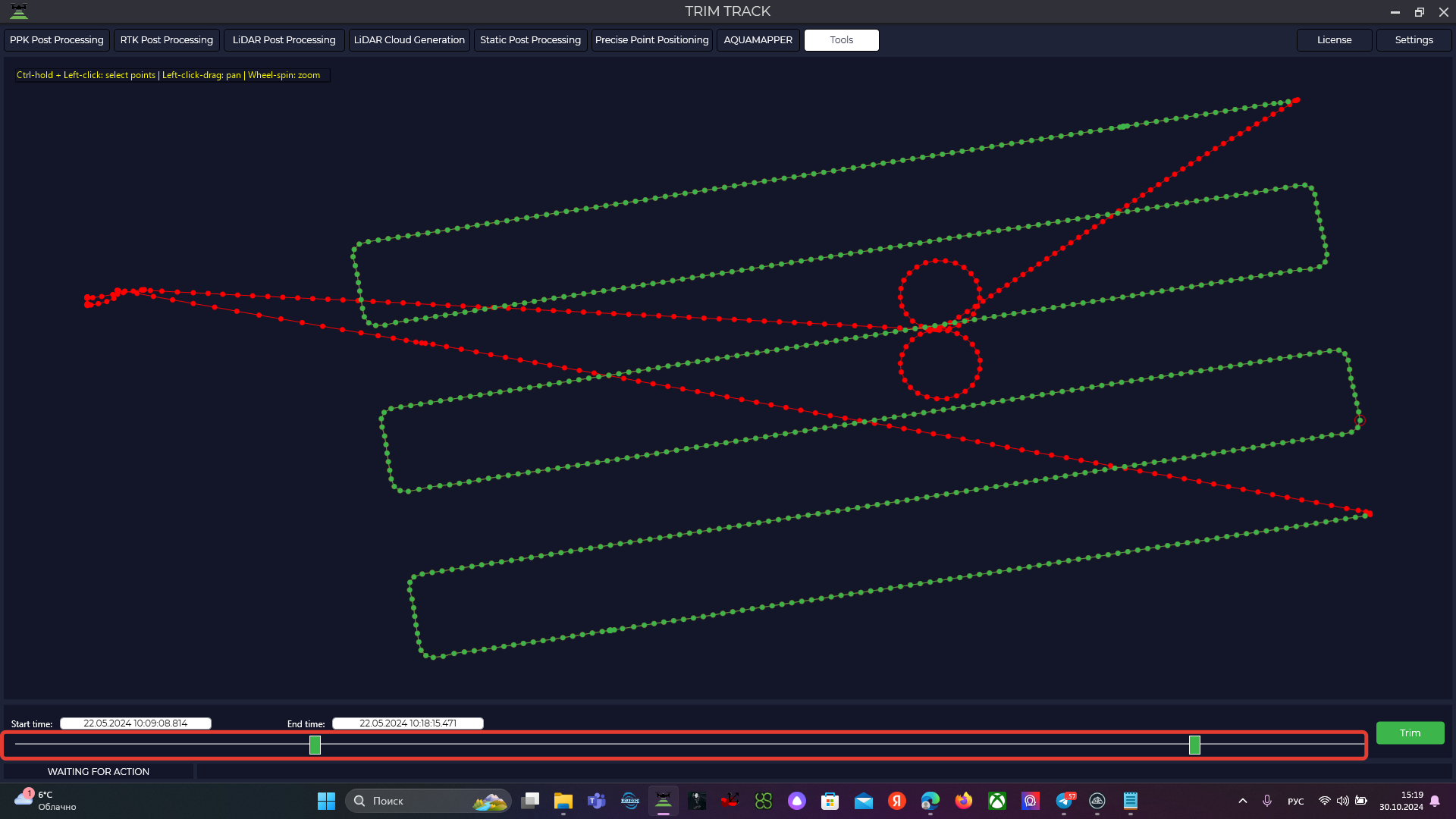
After selecting an area, cut the part you don't want by clicking on "Trim". The trajectory will be saved to a file in the original format.

Merge track files

The module is designed for trajectory stitching followed by point cloud generation in the LiDAR Cloud Generation module.
To start the tool, select Track File Stitching in the Tools, Trim/Stitch tab. Then through the "Add" button select the trajectories to be merged.

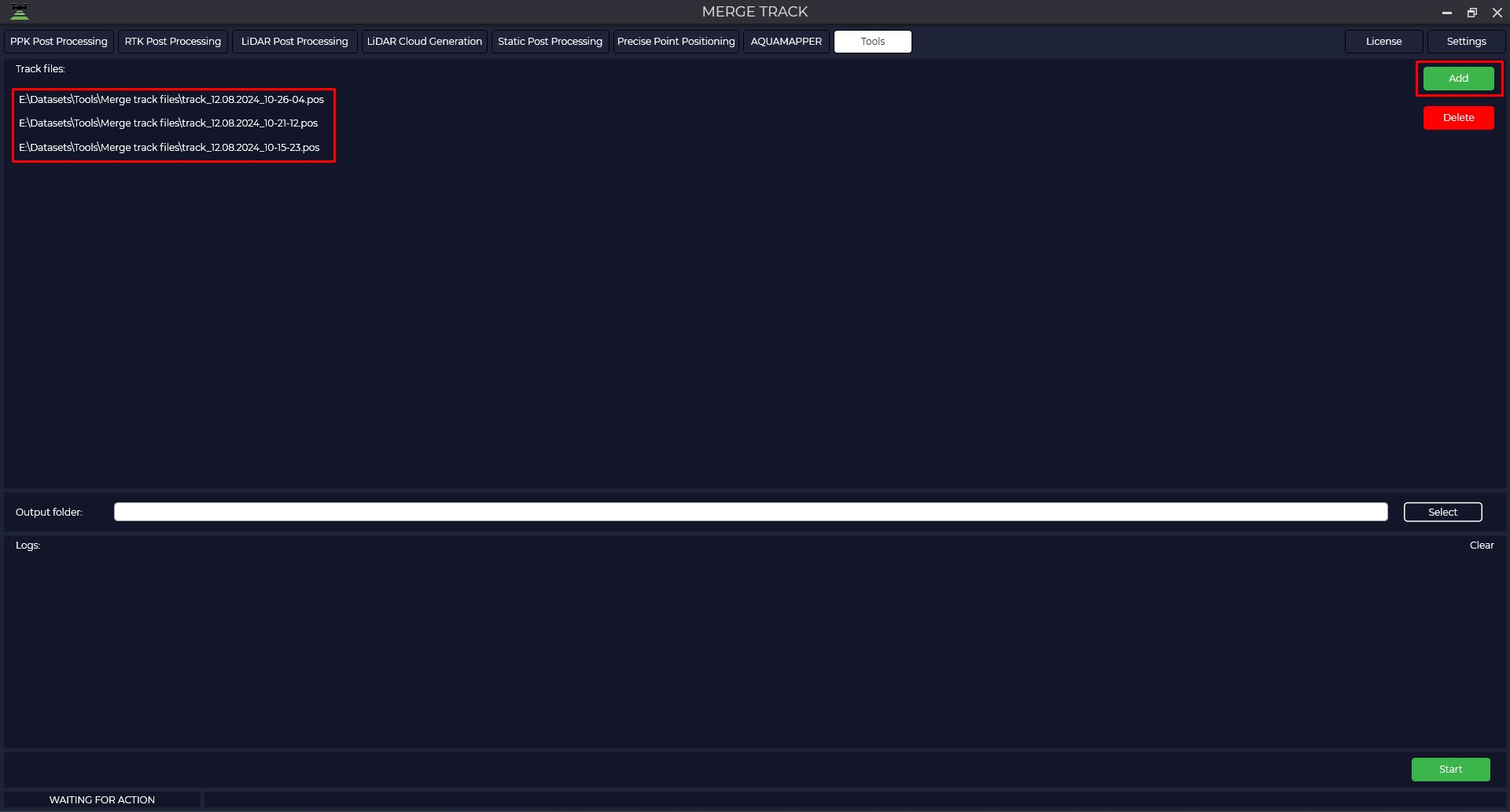
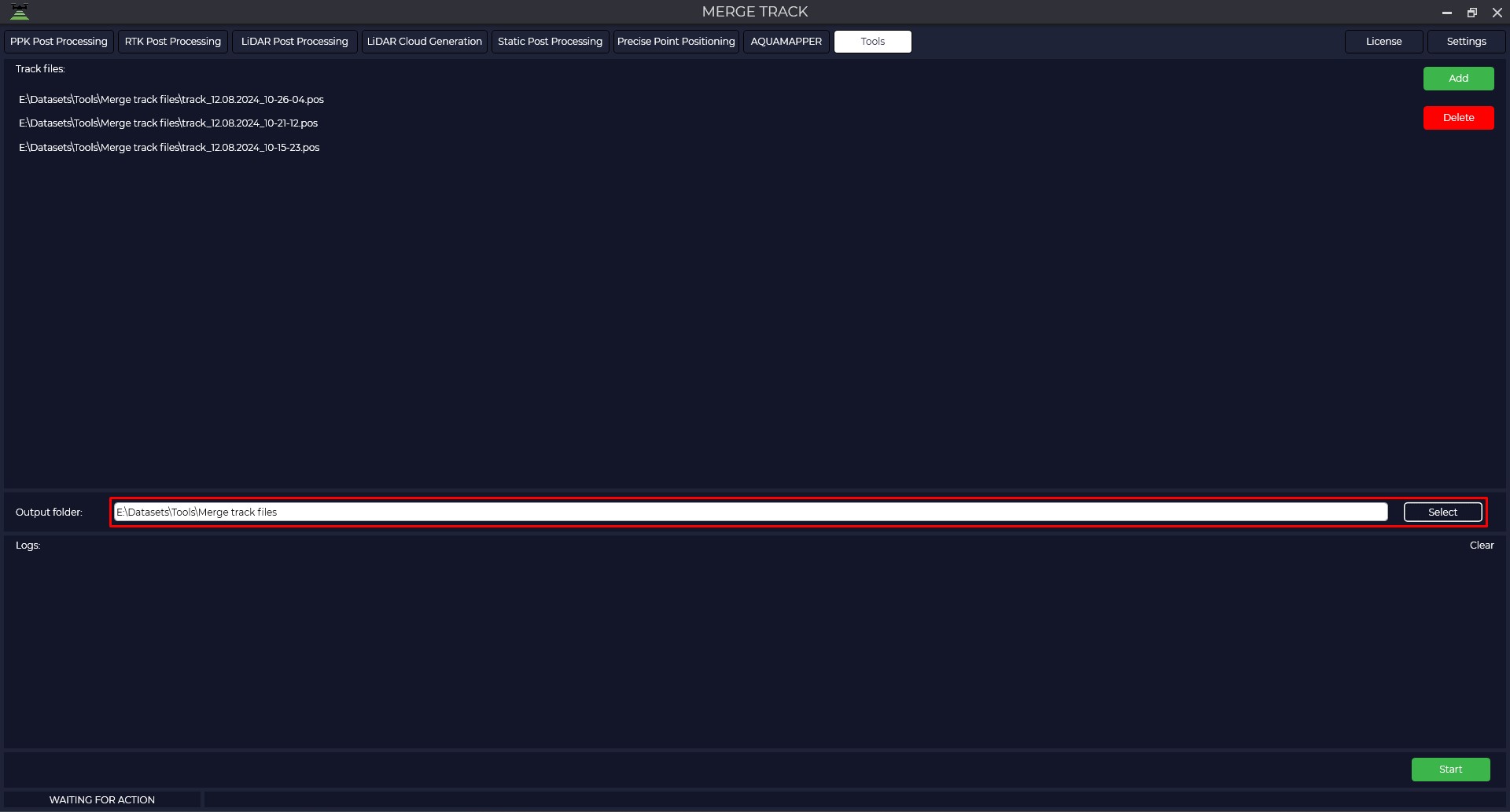
Select the Output folder where to save the merged trajectory and click "Start" to start the process. At the end of the process the program will display a message that everything is ready.

Trim IMR (+GNSS)

You can use the IMR(+GNSS) Trim IMR(+GNSS) tool to eliminate jumps in inertial navigation system (IMU) data when working in conjunction with satellite navigation data.

This tool is useful if after starting trajectory processing the dataset contains an error message - IMU file contains gaps in measurement points! Use the "Trim IMR(+GNSS)" tool to remove the missing sampling time interval.

To start the tool, select IMR(+GNSS) Trim in the Tools, Trim/Stitch tab. Then select the file in *.imr format to be trimmed and the GNSS receiver file.

The program will pre-process the GNSS and if there were any gaps in the IMU data, you will see this on the screen as vertical lines and the designation (Gap).

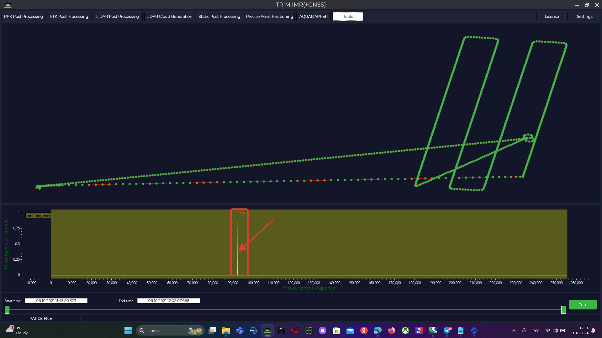
For further correct processing, it is required to exclude outliers from the data.
From the selected file we will need to exclude two skips from processing, therefore the IMU file should be divided into three segments and further processed in three parts. Only one segment is trimmed, so in this case we will need to repeat this procedure three times.

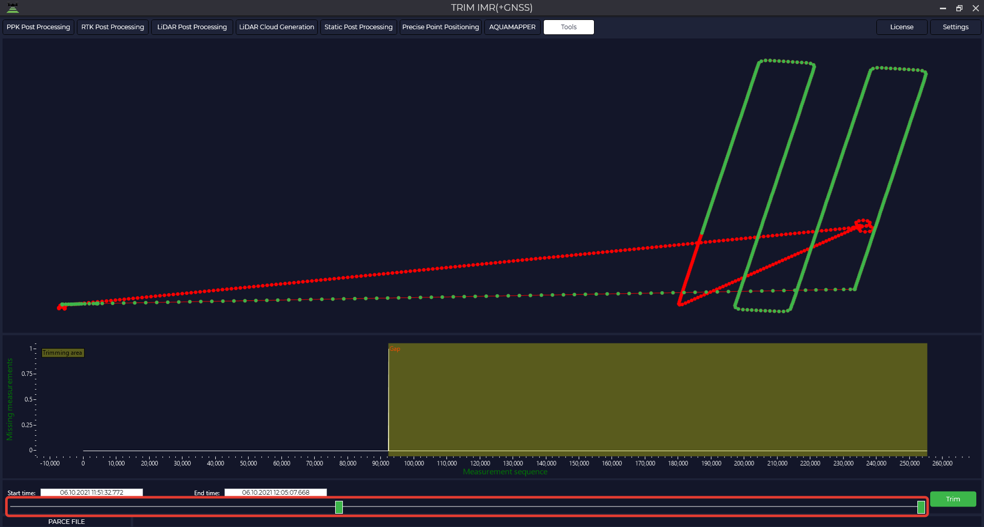
After selecting the desired segment using the sliders at the bottom of the screen, click "Crop". The IMU file will be saved to the folder in its original format at the interval you specified and will be saved to the original folder.

Trim IMR

To eliminate jumps in inertial navigation unit (IMU) data when performing work without satellite navigation data, you can use the IMR Trim tool.

This tool is useful if the dataset contains an error message - IMU file contains gaps in measurement points! Use the IMR Trim tool to remove the missing sample time interval.

To start the tool, select IMR Trim in the Tools, Trim/Stitch tab. Then select the file in *.imr format to be trimmed.

The program will perform pre-processing and if there were any gaps in the IMU data, you will see this on the screen in the form of vertical lines and the designation (Gap).

For further correct processing it is necessary to exclude omissions from the data, therefore the IMU file should be divided into two segments and further processed in two parts. Only one segment is trimmed, so in this case we need to repeat this procedure twice.

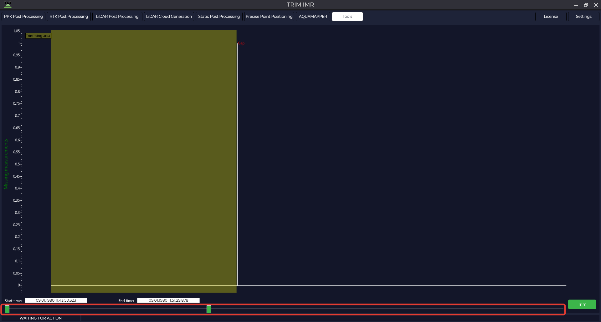
After selecting the desired segment using the sliders at the bottom of the screen, click "Crop". The IMU file will be saved to the folder in its original format at the interval you specified and will be saved to the original folder.

Coordinate converter(One coordinate)

This tool allows to convert data from WGS-84 coordinate system to another one using *.prj file of coordinate system, which is loaded into the program database or using calibration file, which was made before in TOPODRONE Post Processing program. For more details see Calibration.

For example, this tool can help you to convert a base station coordinate from local coordinate system to WGS-84 when processing an area in the LiDAR Post Processing module.

In order to convert one point from WGS-84 coordinate system to any other, you should choose Coordinate Converter in the Tools tab, then One coordinate.

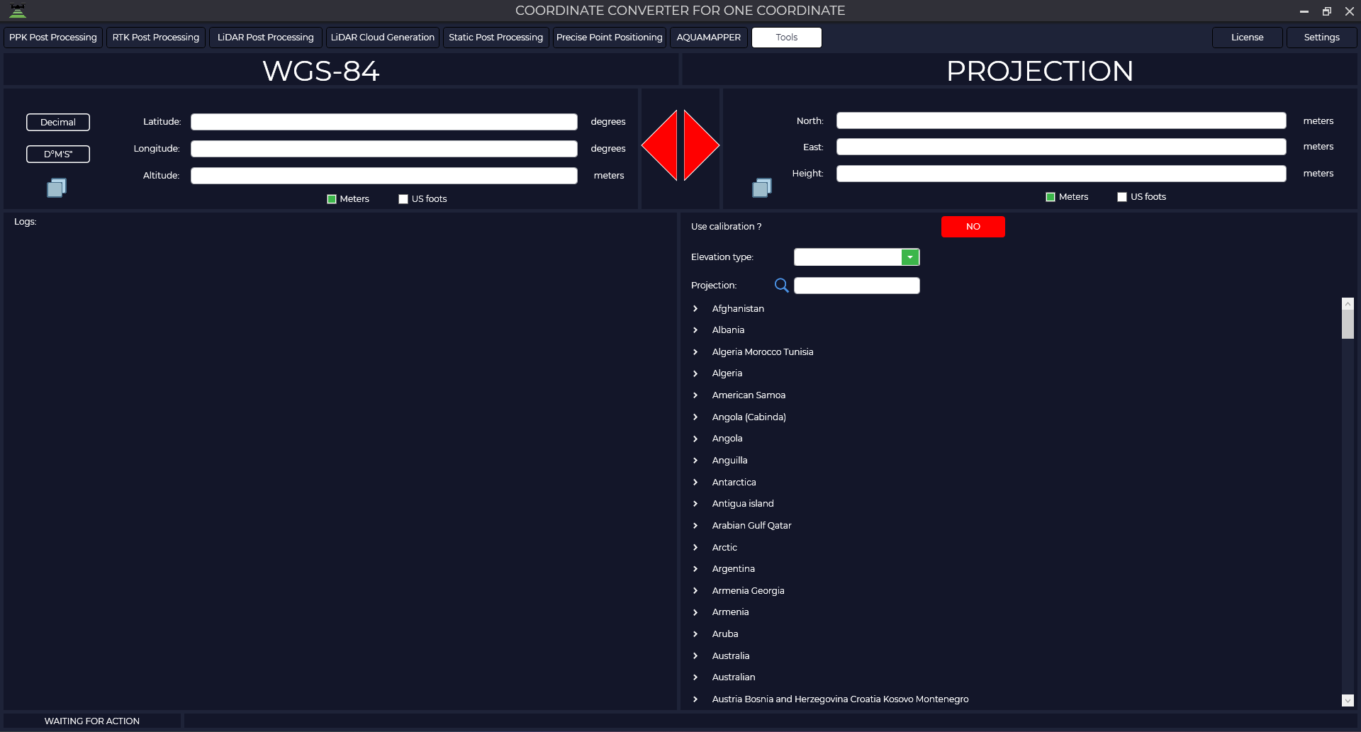
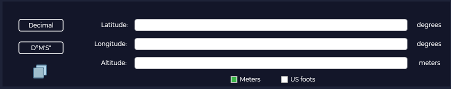
Select the coordinate format (decimal or degrees, minutes, seconds)

Next, select the desired height type.

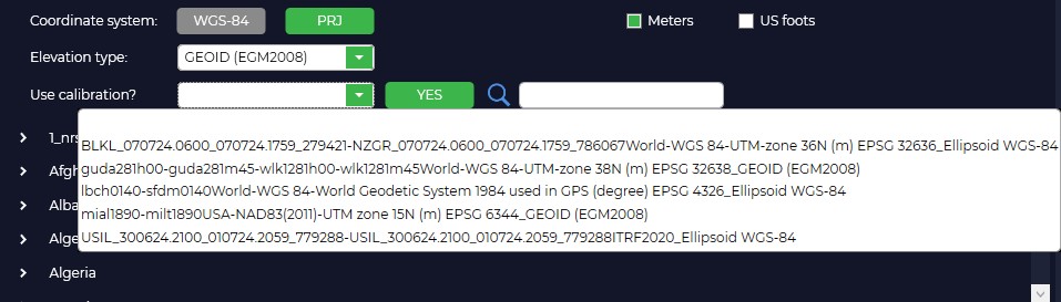
Select the required coordinate system. The required *.prj file can be quickly found using the search bar. The coordinates of the source point must be within the area covered by the *.prj file.

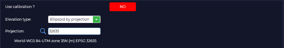
If you have calibrated in the TOPODRONE Post Processing program, press the "NO" button and select your calibration file.

After that, click on the right arrow, which will change its color to green when you hover your mouse cursor over it. Click on the arrow with the left mouse button.

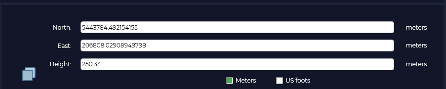
After that, the converted coordinate values of the source point in meters will appear in the right part.

Coordinate Converter(Coordinates from file)

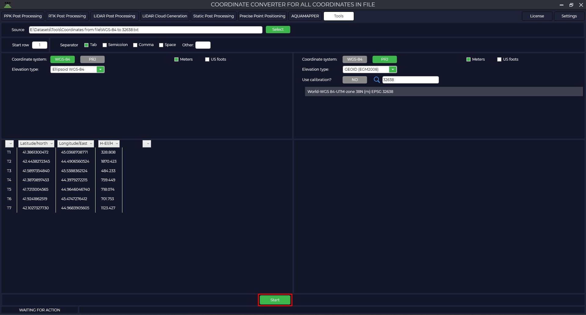
The tool allows you to convert coordinates from one coordinate system to another using the *.prj coordinate system file loaded into the program database or the calibration file created earlier in the TOPODRONE Post Processing program. More details about this process can be found in the "Calibration" section. To convert a coordinate catalog from one coordinate system to another, go to the "Tools" menu and select "Coordinate Converter", then "Coordinates from file".

In the Source section, specify the coordinate catalog file you want to convert, the import start line, and the coordinate separator type.

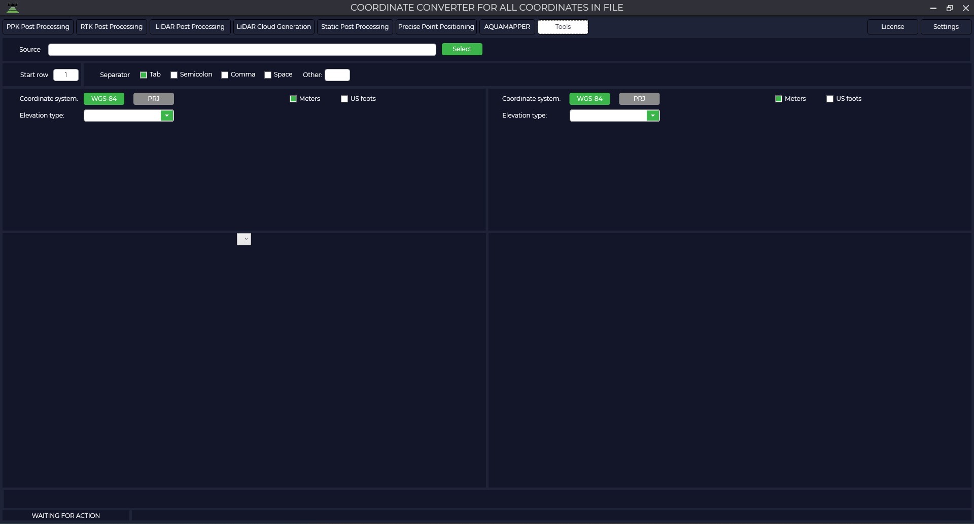
Select the coordinate system and elevation type of the original coordinate catalog.

Determine whether the columns match the values.

Specify the coordinate system and elevation type of the target coordinate catalog.

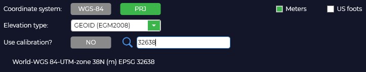
If you have calibrated in the TOPODRONE Post Processing program, press the "PRJ" button, then press "NO" and select your calibration file.

After pressing the "Start" button, the right window will display the coordinate catalog in the selected coordinate system. If necessary, click the "Save" button and save the new file.

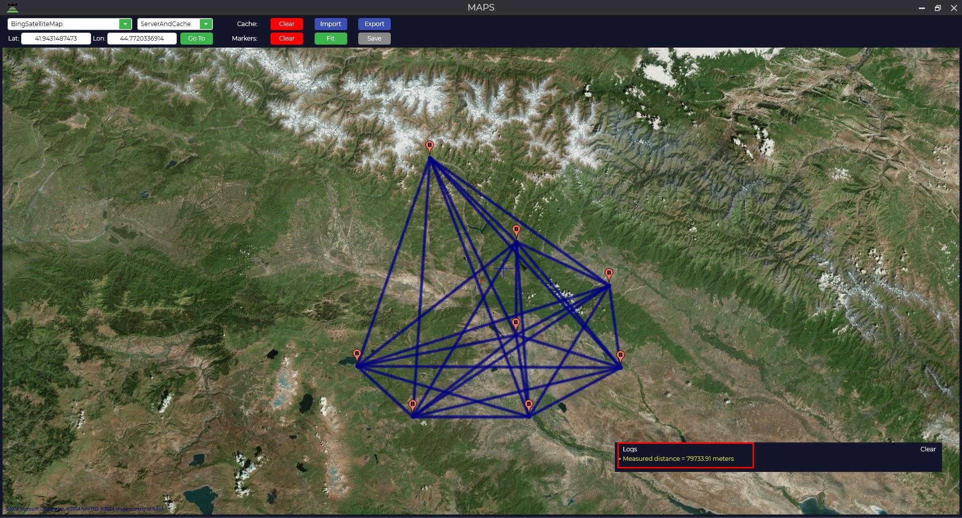
Maps

The "Maps" module is designed to display loaded static observations and vectors at all stages of data processing. To launch the module, go to the "Tools" tab and click the "Maps" button. Important: for correct display of observation points, the map window should be opened when loading files. If this condition has not been met, you should re-download the data. An additional function of the module is to measure the distance between two points on the map. To do this, press the "Ctrl" key and select two points in the map area with the left mouse button. The value of the measured distance will be displayed in the log window.

GNSS data converter

The module is based on the open source software RTKLIB, this module is designed to convert raw observation files from Global Navigation Satellite System (GNSS) receivers into RINEX format. The module supports data formats from the following GNSS chip manufacturers: U-blox, ComNav, NovAtel, Hemisphere, Javad, Trimble, as well as the common *.YYO format, where YY is the year of observations.
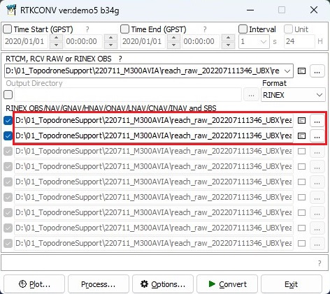
To convert data to *.obs format, perform the following actions: Go to the "Tools" tab and select "GNSS Data Converter" in the RINEX section. Specify the file to be converted to *.obs format.

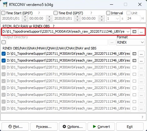
The lower part of the window displays the files to be exported.

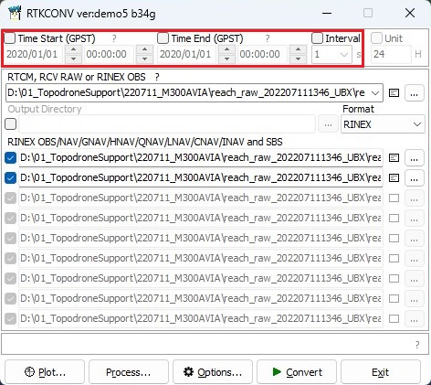
If necessary, time-limit the file by specifying the date and range of operation, and change the frequency of the final file write.

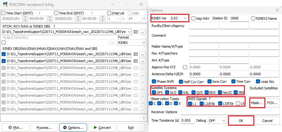
Click on the "Options..." button and select the RINEX version, satellite constellations, operating frequency or specific satellites. Then click on the "OK" button.

Click on the "Convert" button to have the program convert your file to RINEX format with your parameters.

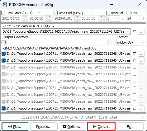
After converting the file, click on the "Plot..." button to evaluate the quality of your data. For more information about data quality analysis, see Appendix B.

RINEX merger

This function is designed to merge measurement files received from different receivers of the global navigation satellite system into one file. It is especially useful when the reference base station provider divides files into time slots when downloading data.
Follow the steps below to merge the files: Go to the Tools tab and select Merge under RINEX.

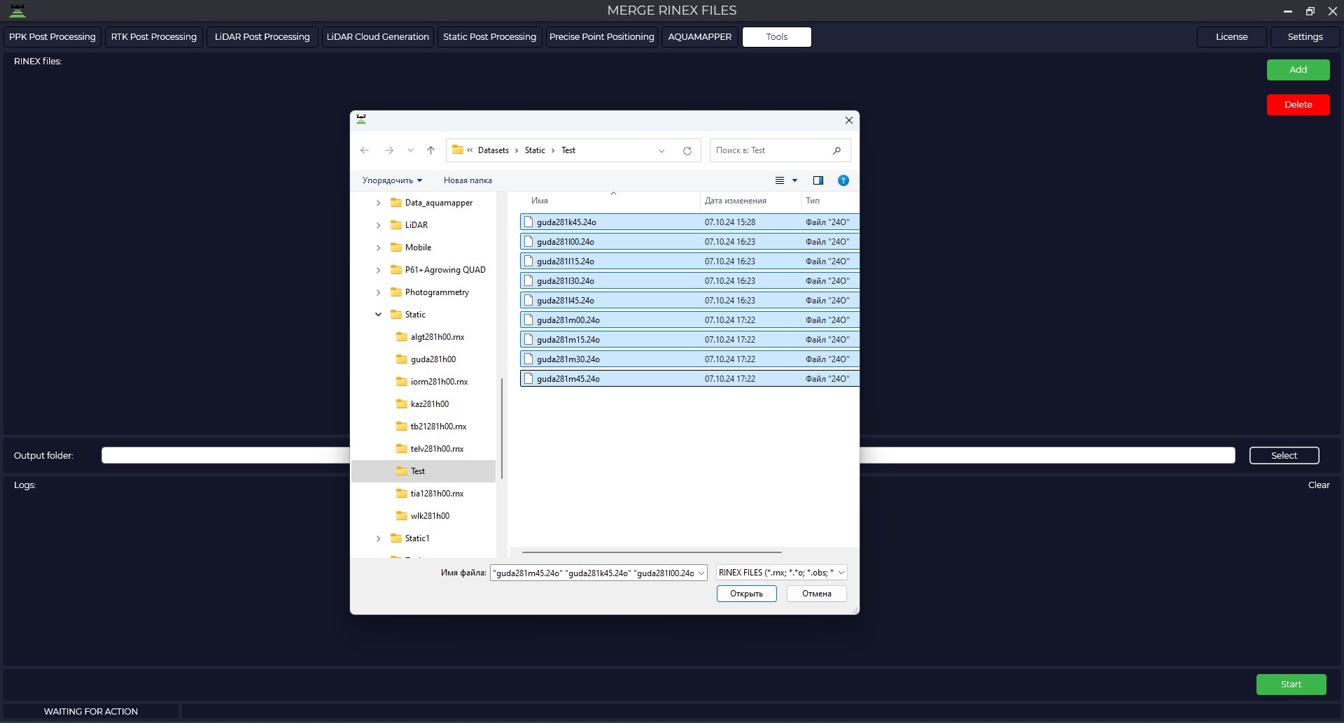
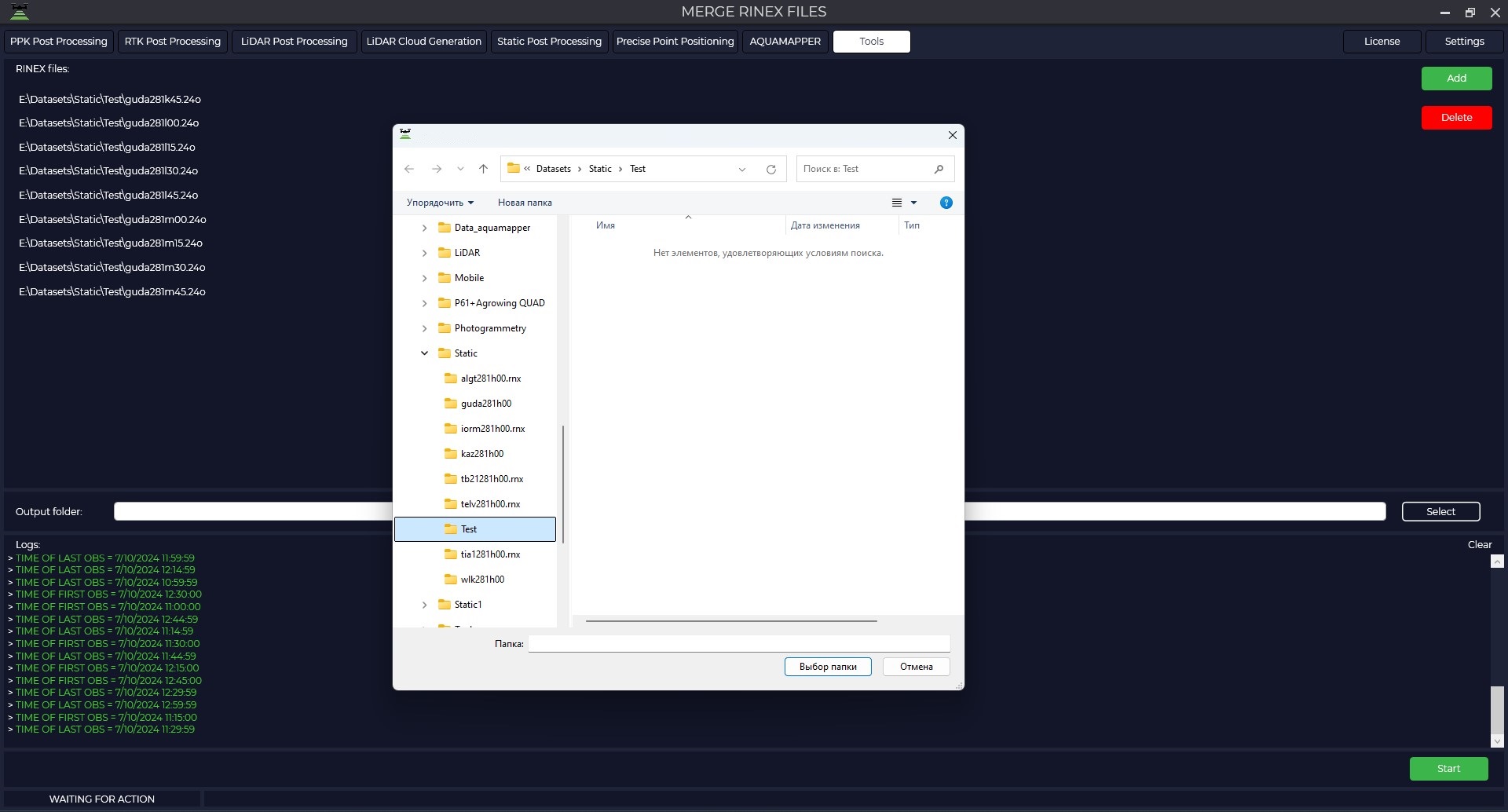
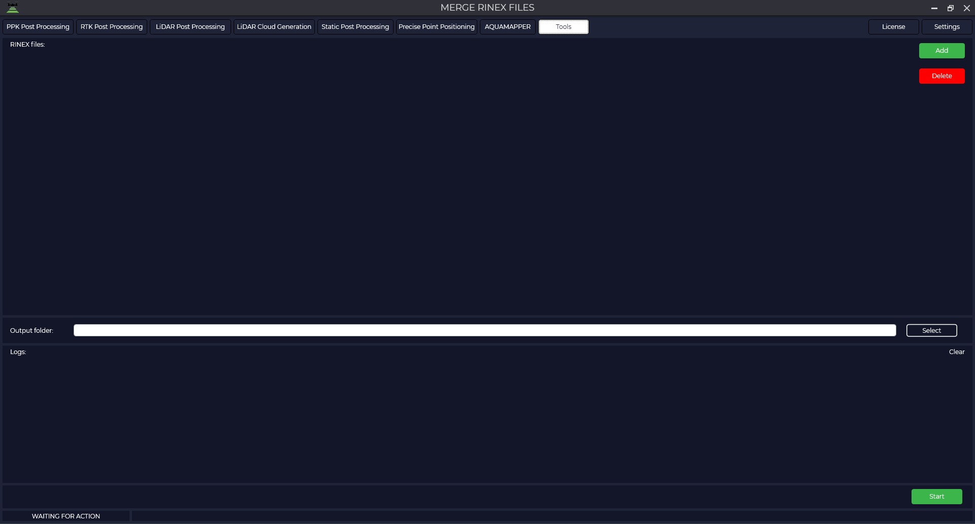Click the "Add" button to add measurement files and select the required files in *.rnx, *.**o and *.obs formats.

The "RINEX files" window will display the downloaded files, and the "Logs" window will display information about the recording time, antenna type, and receiver coordinates that the program reads from your files.

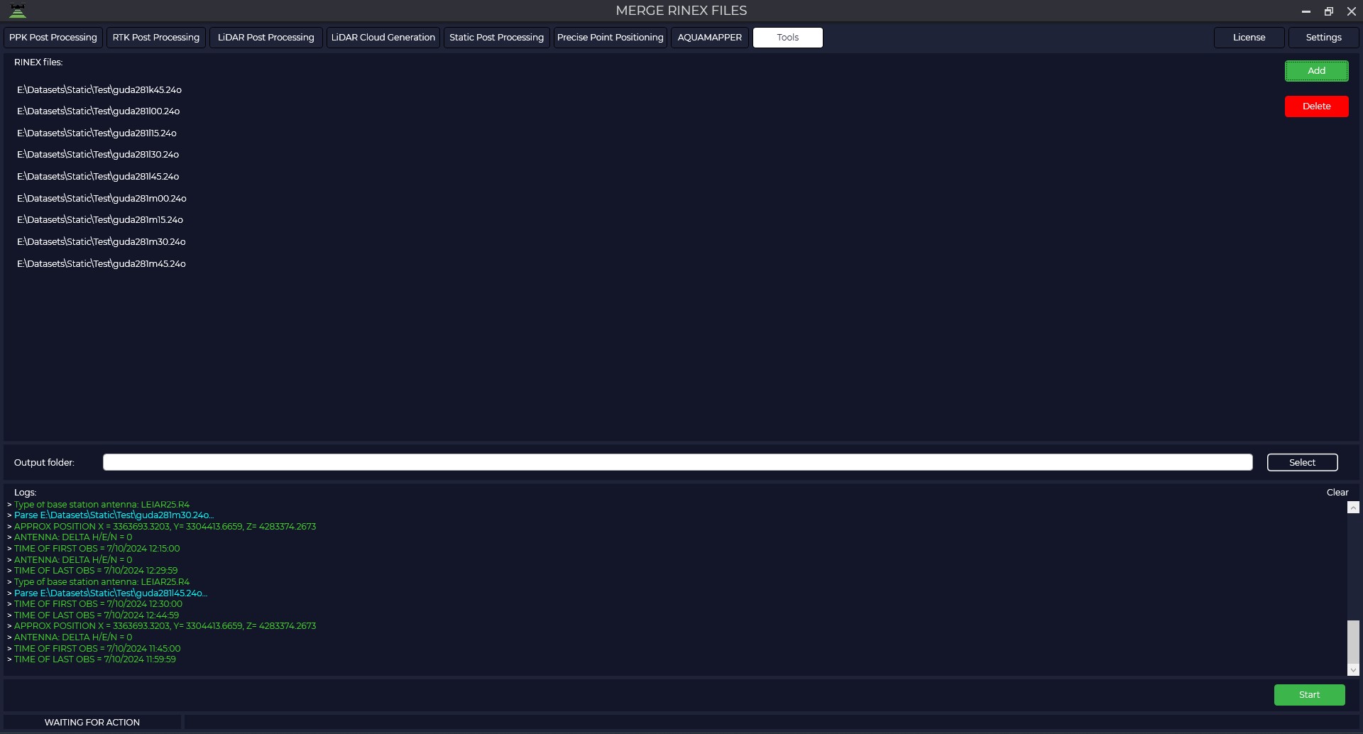Specify the path to the folder where you want to save the merged file.

Click on the "Start" button to have the program merge all files and save to the previously specified folder.

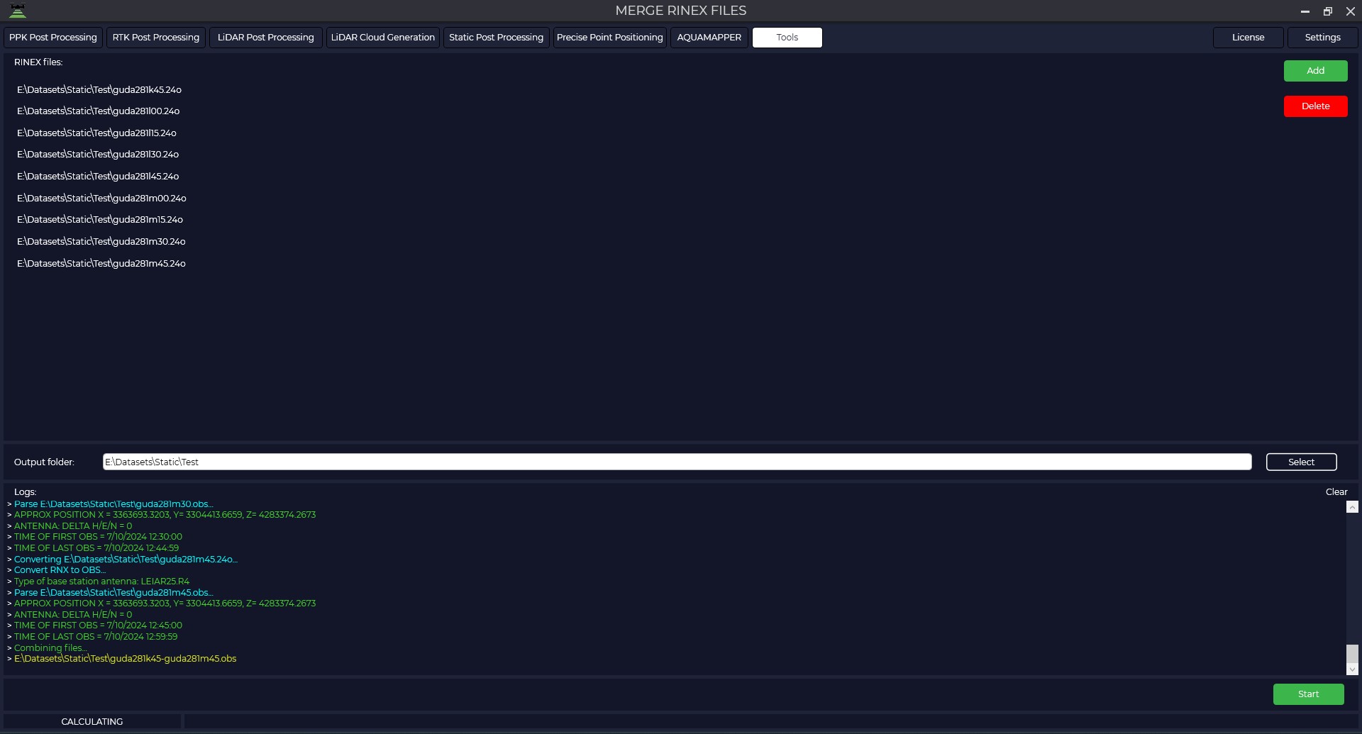After the file merge operation is successfully completed, you can use the resulting file for further data processing.

Satellite filtering

This module allows you to exclude certain satellite constellations or specific satellites from the observation file, which may be necessary to improve data quality.

Follow the steps below to filter satellites: Go to the "Tools" tab and select "Rinex", then "Satellite Filtering".

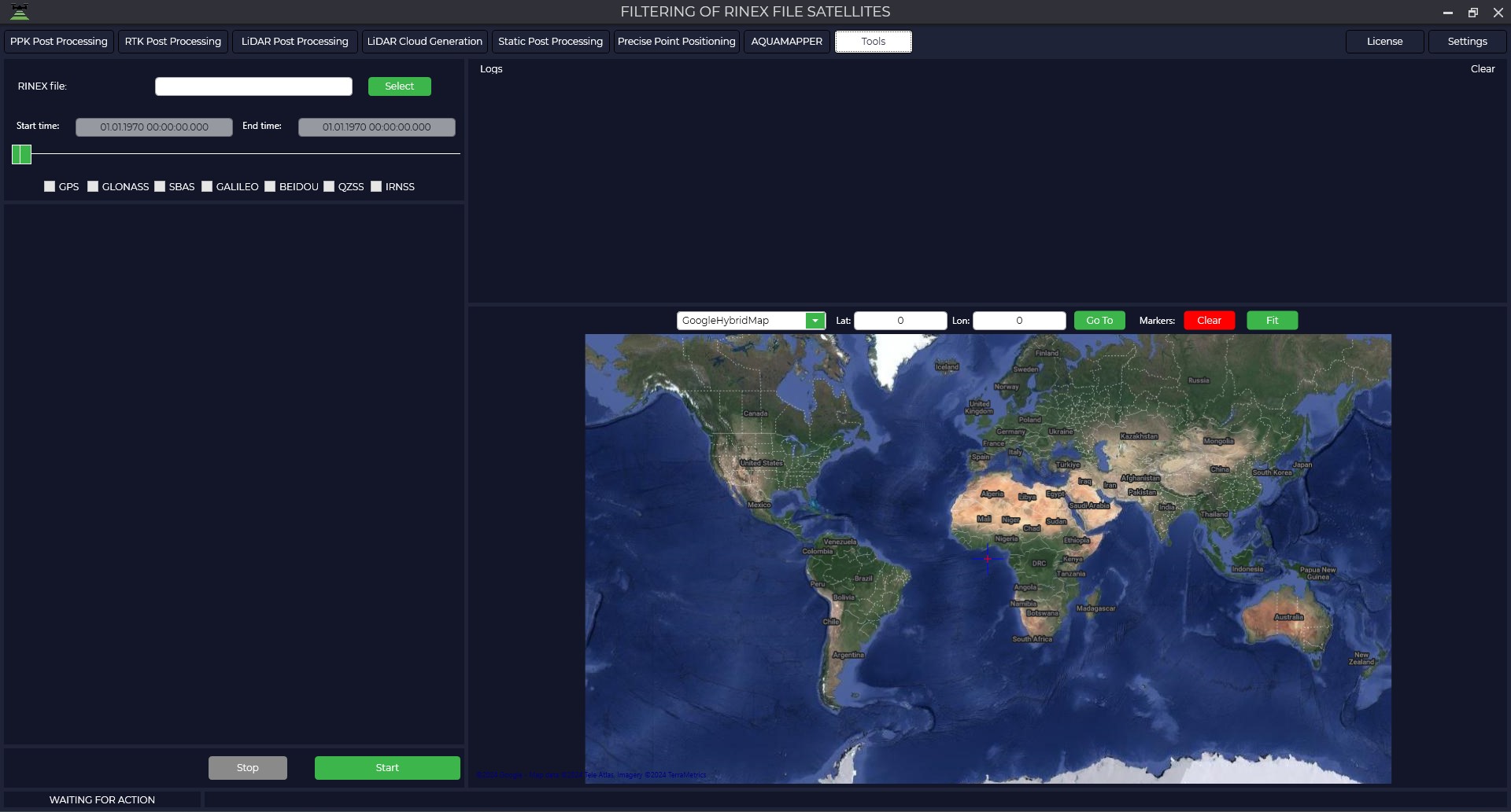
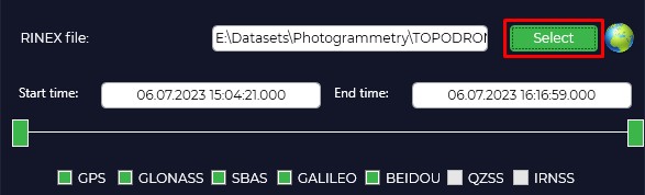
In the upper left part of the RINEX file window click the "Select" button and specify the raw observations file in *.obs format.

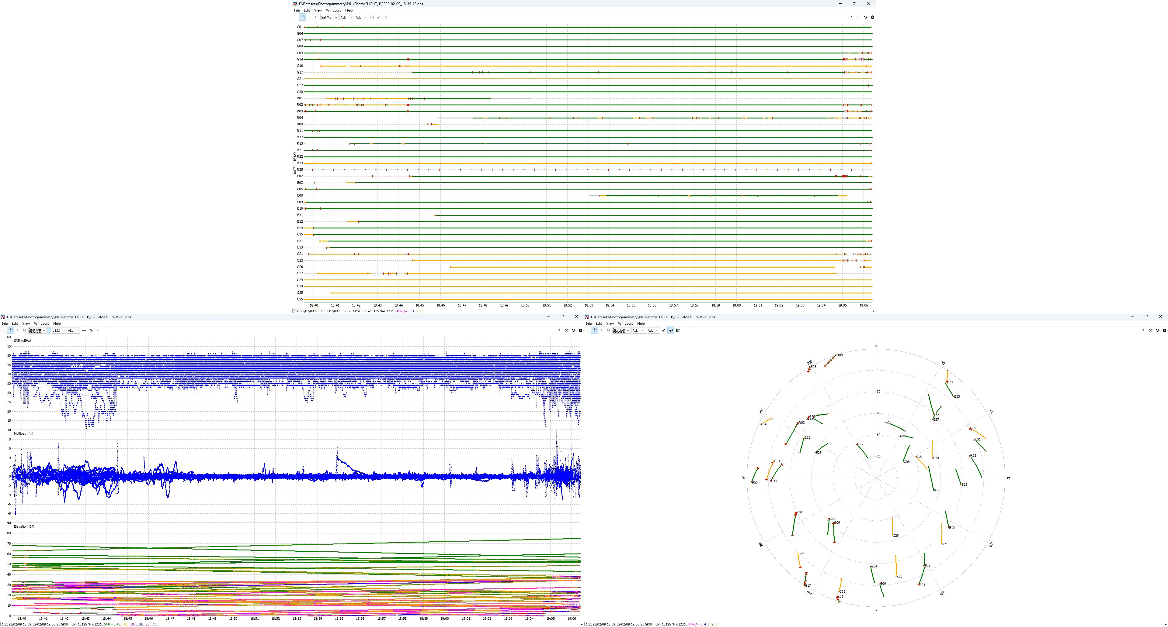
Click on the icon to view the signal quality to open the "Plot" window, which allows you to understand which satellites may be interfering with data processing. For more information about data quality analysis, see Appendix B.

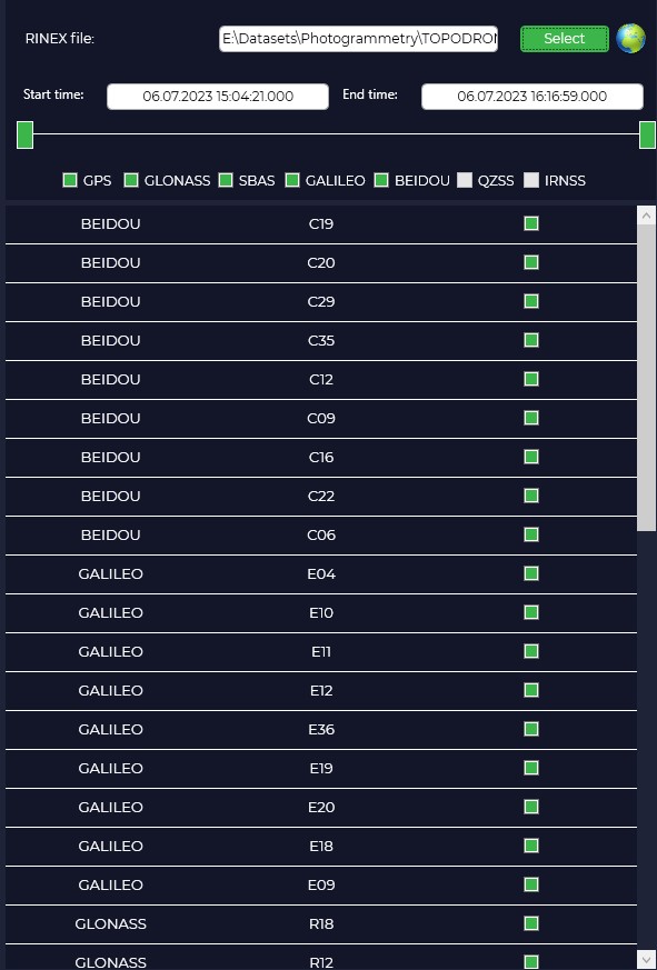
Move the sliders left and right if necessary to change the start and end time of the file.

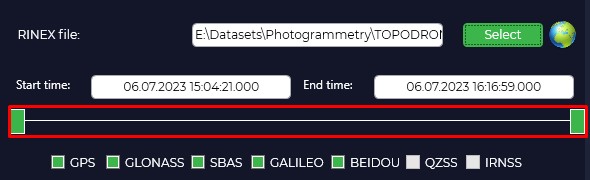
Uncheck the required checkboxes if you want to exclude certain satellite constellations (GPS, GLONASS, GALILEO and BEIDOU) or specific satellites.

Press the "Start" button. The program will save the new file, excluding the selected satellites from it.

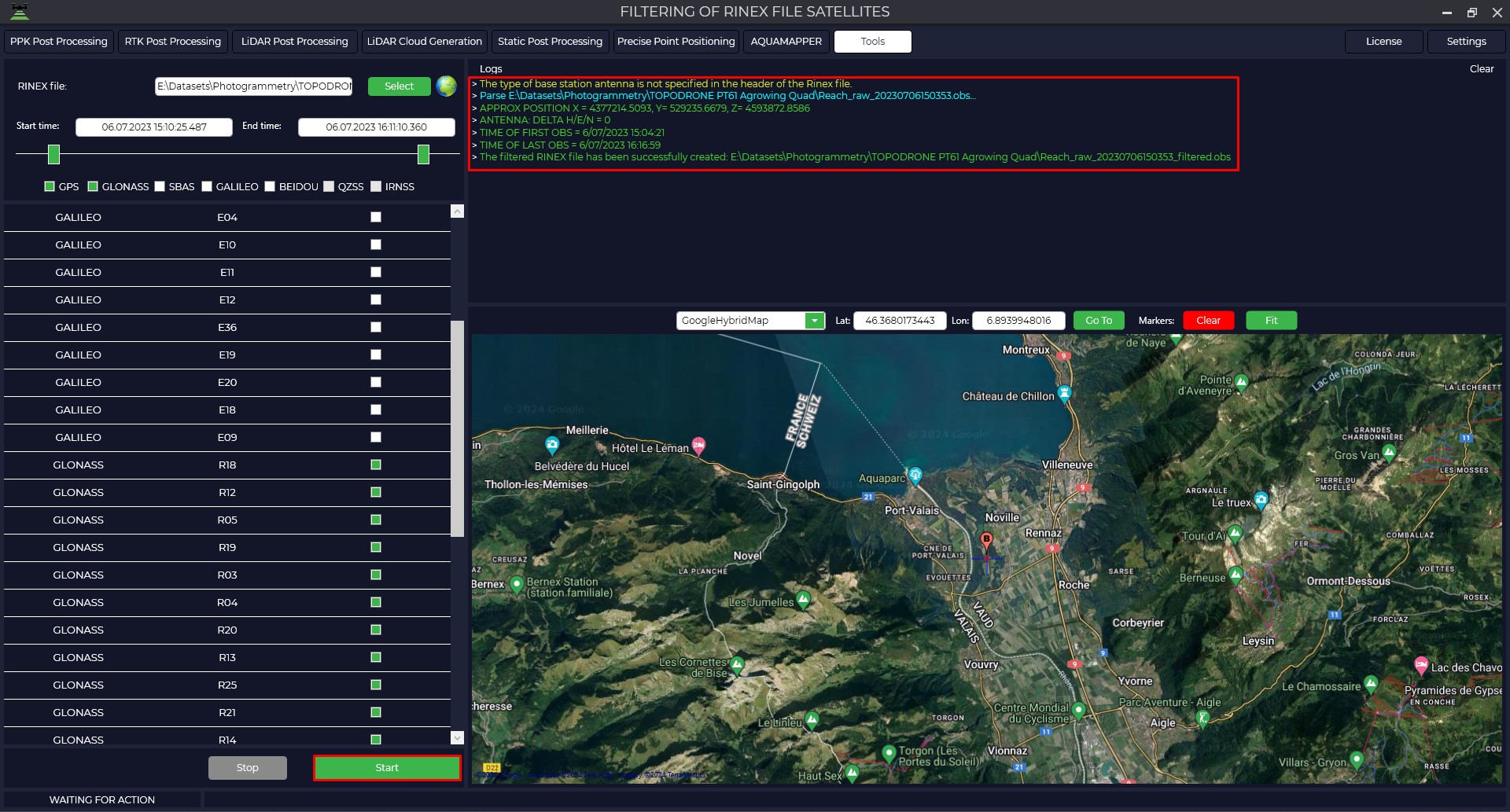
Once the satellite filtering operation has been successfully completed, you can use the resulting file for further data processing.

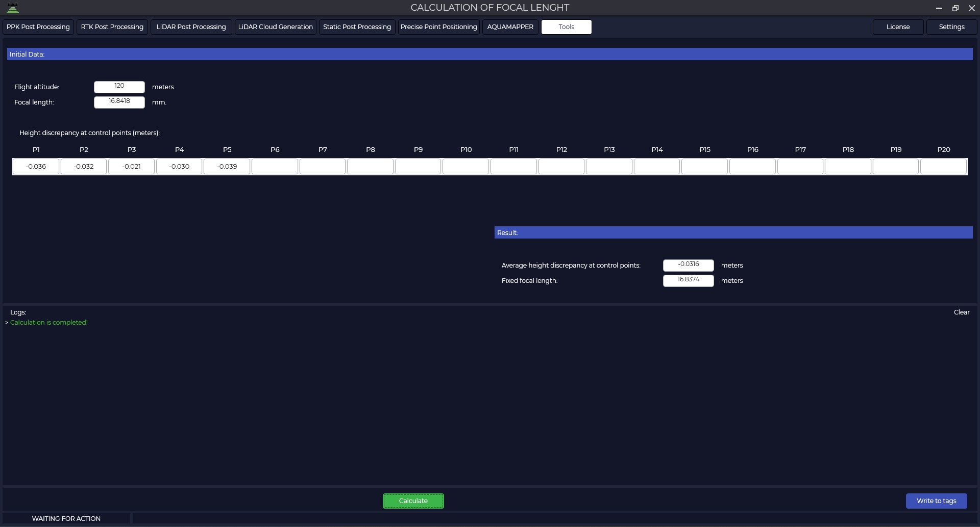
Calculating the focal length

This tool is not directly related to GNSS data processing, but it helps to calculate the focal length of the camera, which is necessary for data processing in photogrammetric programs.
Instructions for calculating the focal length:

1. Click the Tools tab and select Focal Length Calculation.

2. In the opened window specify the following parameters: flight altitude of your aircraft, previously obtained focal distance in millimeters (from the result of aerotriangulation in photogrammetric software) and error values by height of your control points.

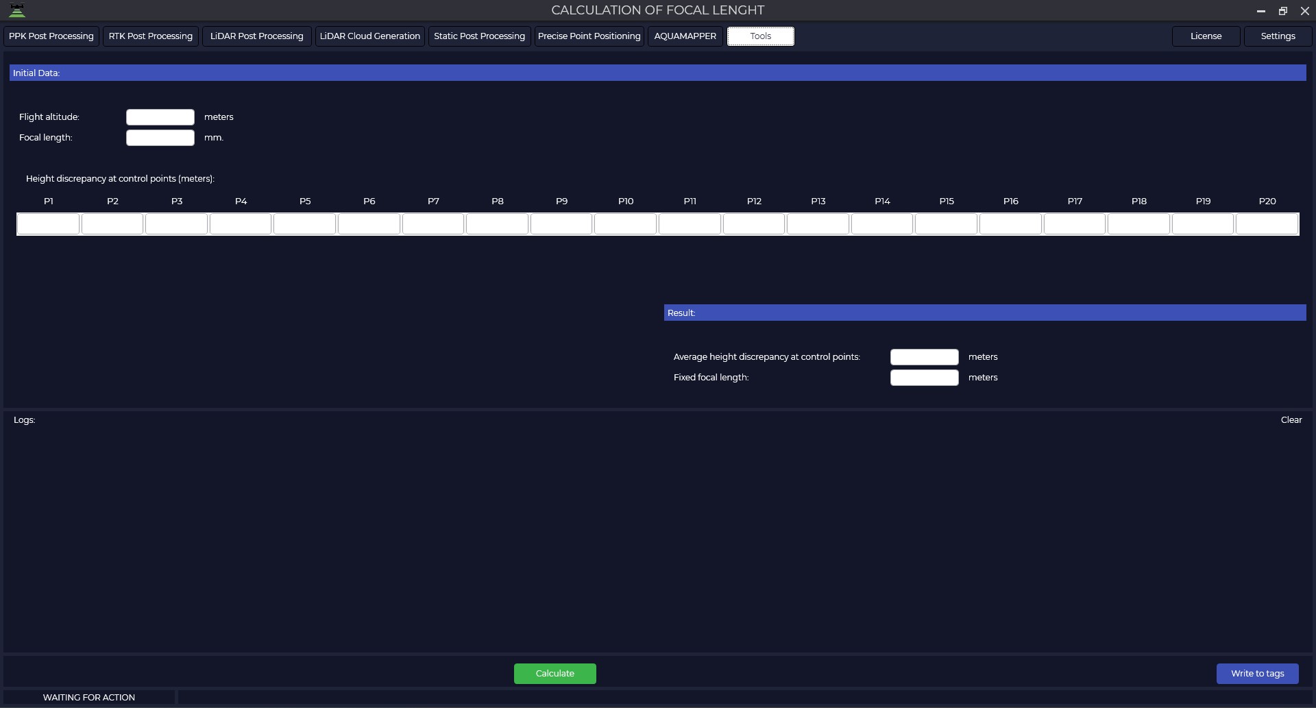
3. Click the "Calculate" button. The program will calculate average height error and focal length, which can be used in photogrammetric programs.

4. If necessary, the new focal length can be written to the EXIF tags of your photos by clicking the "Write to Tags" button. This will help in further photogrammetric data processing.

5. Specify the folder with the photos.

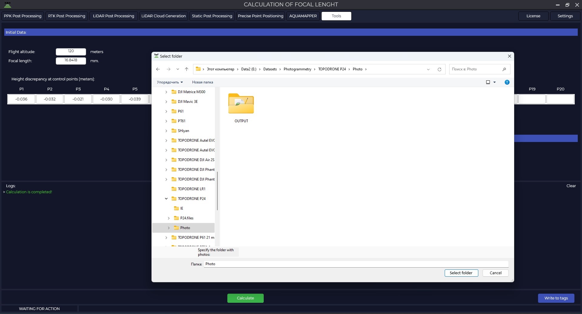
6. The program will write the new focal length to all photos in the specified folder.

The program replaces the focal length in the original files without creating copies of the photos.