TOPODRONE Post Processing
- TOPODRONE Post Processing software installer
- TOPODRONE Post Processing software installer
- Starting the program and entering the key
- License renewal request
- Software running w/o Internet connection
- Downloading installation files
- Changes in licensing of the software "TOPODRONE Post Processing"
- TPP v.1.5.2.1 updated 27.07.2025
- TPP v.1.5.1.4 updated 07.03.2025
- TPP v.1.5.1.3 updated 25.01.2025
- TPP v.1.5.1.2 updated 28.12.2024
- TPP v.1.4.5.0 updated 12.11.2024
- TPP v.1.4.4.4 updated 04.11.2024
- TPP v.1.4.4.2 updated 02.10.2024
- TPP v.1.4.4.1 updated 10.09.2024
- TPP v.1.4.4.0 updated 13.08.2024
- TPP v.1.4.3.0 updated 30.07.2024
- TPP v.1.4.2.0 updated 20.06.2024
- TPP v.1.3.3.4 updated 23.04.2024
- TPP v.1.3.3.0 updated 05.04.2024
- TPP v.1.3.2.2 updated 17.03.2024
- TPP v.1.2.0.1 updated 23.11.2023
- TPP v.1.2.0.0 updated 20.11.2023
- TPP v.1.1.17.0 updated 13.11.2023
- TPP v.1.1.16.1 updated 1.11.2023
- TPP v.1.1.16.0 updated 30.10.2023
- TPP v.1.1.15.0 updated 04.10.2023
- TPP v.1.1.14.0 updated 20.09.2023
- TPP v.1.1.13.0 updated 29.08.2023
- TPP v.1.1.12.0 updated 22.08.2023
- TPP v.1.1.11.1 updated 08.08.2023
- TPP v.1.1.9.1 updated 24.06.2023
- TPP v.1.1.9.0 updated 04.06.2023
- About
- System Requirements
- Installation, activation and deactivation of the TOPODRONE Post Processing software
- Preparation of initial data
- PPK Post Processing
- RTK Post Processing
- LiDAR Post Processing
- LiDAR Cloud Generation
- Static Post Processing
- Precise Point Positioning
- AQUAMAPPER
- Tools
- Filters LAS/LAZ
- Ground classification
- LAS/LAZ Insta 360 Coloring
- PRJ editor
- Viewing the point cloud
- Data archive GNSS
- Track trimming
- Merge track files
- Trim IMR (+GNSS)
- Trim IMR
- Coordinate converter(One coordinate)
- Coordinate Converter(Coordinates from file)
- Maps
- GNSS data converter
- RINEX merger
- Satellite filtering
- Calculating the focal length
- Settings
- General
- Aerial photography
- Lidar scanning
- Laser scanner track file structure
- Laser Scanner Sensor Beam Calibration
- AQUAMAPPER
- Appendix A. Manual matching of photographs and timestamps.
- Appendix B. Analysis of GNSS data.
- Release Notes
TOPODRONE Post Processing software installer
TOPODRONE Post Processing software installer
Download TOPODRONE Post Processing software installer
About the TOPODRONE Post Processing software installer
TOPODRONE Post Processing software installer is a compact application designed primarily to automate the process of downloading TOPODRONE Post Processing software distributions. This application greatly simplifies the management of software updates and versions, providing users with access to the latest versions and enhancements.
In addition to the basic download function, the program has the following features:
1. Downloading current software versions: The downloader provides the ability to download new versions of TOPODRONE Post Processing that have been released during the upgrade license period. This allows users to stay on the cutting edge of technology and utilize the latest enhancements and patches.
2. View Change Records (Changelog): The built-in Change Viewer provides users with information on all updates released as part of new distributions. This provides a quick overview of innovations, bug fixes, and functionality improvements, which is especially useful for assessing the impact of updates on workflows.
3. Upgrade License Renewal: The software installer offers an easy and affordable way to extend the validity of license key upgrade control, allowing users to continue using the latest software features without a service interruption.
4. Software Version Upgrade: the software installer also provides functionality to perform upgrades to more advanced versions of the software: PRO or Expert. These versions offer advanced features and tools for deeper analysis and data processing.
Download TOPODRONE Post Processing with license key
Software initialization: when the software installer is launched, a loader window opens where the user can start the installation and activation process.
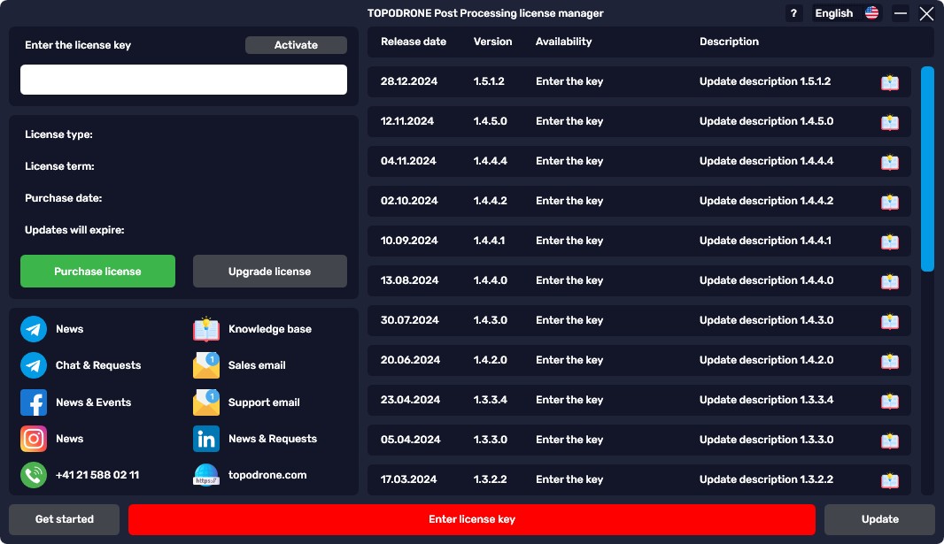
Entering the license key: If you have a valid license key, you must enter it in the designated field marked "Enter the license key". Then click Activate to view the available versions of TOPODRONE Post Processing.
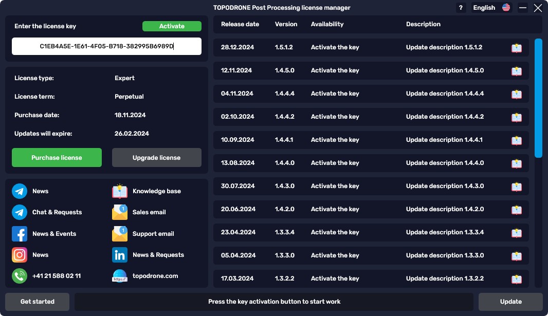
The license key consists of 36 characters and has the following format: ********-****-****-****-************. If your key consists of 19 characters and is presented in the form ****-****-****-****-****, it indicates that it belongs to the previous licensing system and is not suitable for current software versions. To get a new license key, it is recommended to use the “Support mail” button or send a request to e-mail, specifying the name of the equipment used and the name of your organization.
Displaying available versions: After successfully entering the license key, the right side of the program interface will display information about the software versions available for download. Versions available for download and installation within the current license key validity period are highlighted in blue, while versions that require license extension are highlighted in gray.
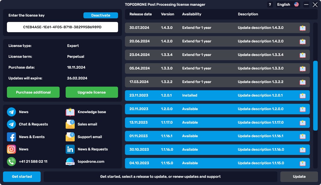
Software update: To update the TOPODRONE Post Processing software, select the appropriate line in the list of available versions, which will be highlighted in green color, then click the “Download” button and specify the path to the folder to save the downloaded file.
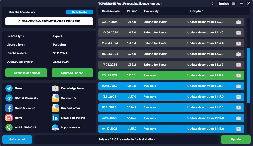
Download Progress Display: The bottom of the window will display the download progress percentage, allowing the user to track the process.
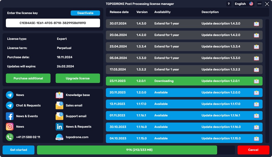
Installation Process: After the download is complete, install the software. In the installer window that opens, follow the standard procedures to complete the TOPODRONE Post Processing software installation.
Activation and deactivation of TOPODRONE Post Processing program
After successful installation, launch the program and click "Get Started". The program will be activated and ready for use, allowing you to successfully perform tasks related to post-processing data and implementing the functionality provided by the TOPODRONE system.
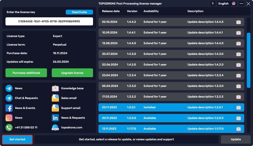
These steps provide a clear understanding of the software installation and activation process, making it much easier for users to interact with the product.
To deactivate the software, click on the “Revoke” button. Only after this action you will be able to activate another device.
When you run the program for the first time, the following message may appear: “To run this application, you must install .NET Core. Would you like to download it now?” It is necessary to download and install this library.
Sending a License Renewal Request
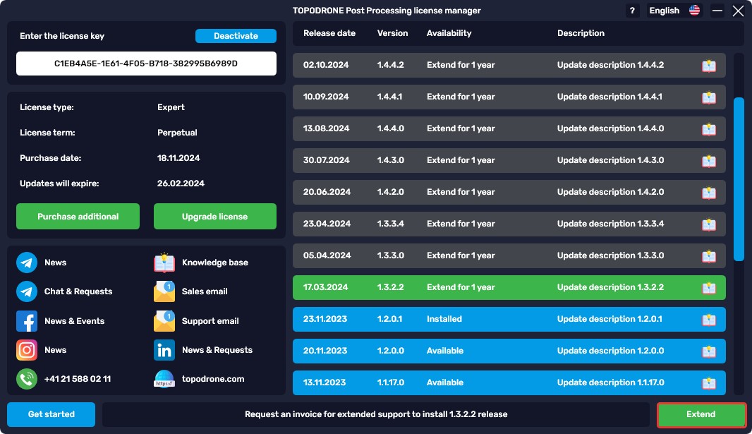
During software installation, the user is provided with information about the current version of the program and available versions for updating.
|
|
Available version |
|
|
Selected version |
|
|
Versions are not available for the current key, renewal is required |


If the current version of the software cannot be updated, you must initiate the license renewal process. To do this, the user is asked to select a new target version and request an invoice for payment by filling out the feedback form.
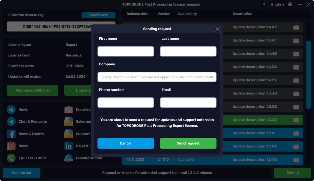
If you have a license key, enter it in the designated field for activation and click "Activate".
After successful verification of the license key, information about available license modifications will be displayed, including the possibility of purchasing a new version or upgrading the current version of TOPODRONE Post Processing to a more advanced one.
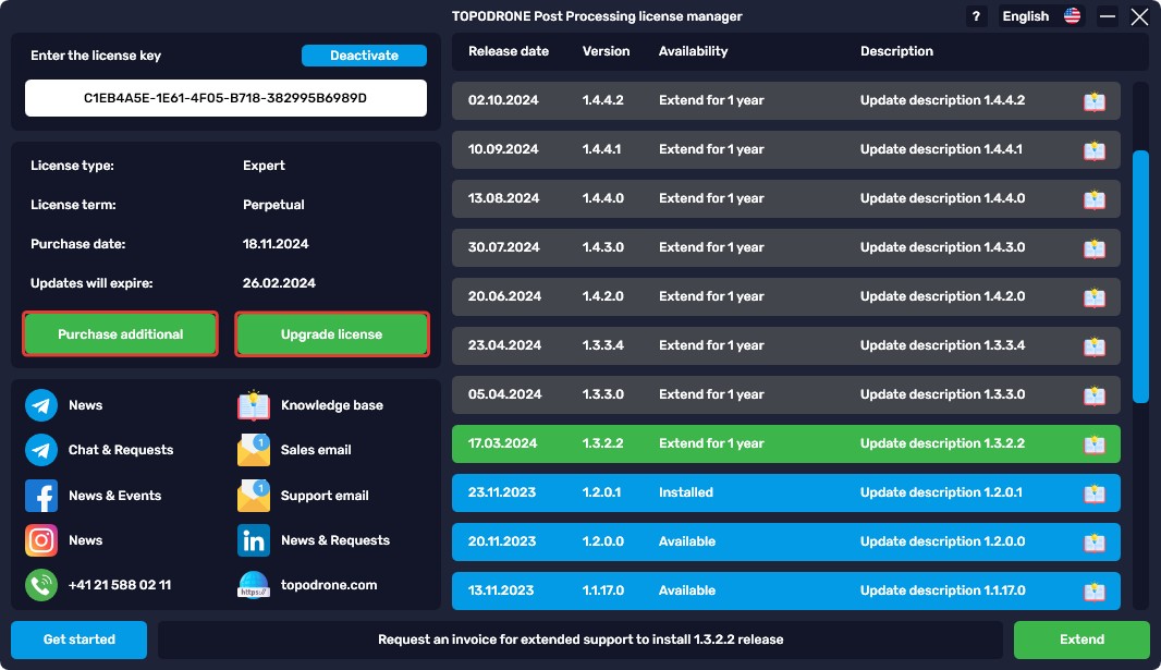
In the left panel, the user must select one of the options: "Buy a new one" or" Improve the current one " to get acquainted with the update capabilities. As a result of this action, information about software versions will be displayed with a list of available modules for each version.
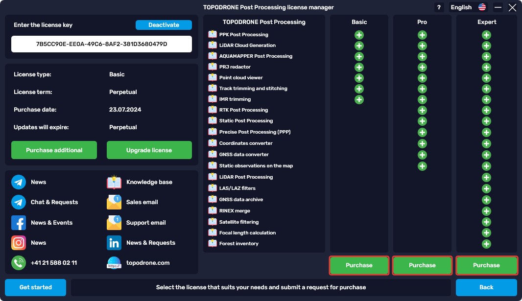
At the next stage, select the appropriate " Buy " action and fill out the feedback form.
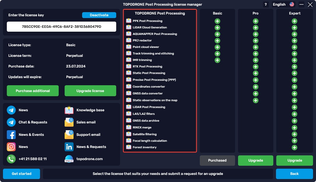
The TOPODRONE Post Processing loader also contains up-to-date information about all available modules in the program. Each version includes a specific set of modules grouped under three licenses: Basic, Pro, and Expert.
To get detailed information about each module, you can click on its name, which will redirect you to the corresponding section of the TOPODRONE knowledge base with a full description of its characteristics and functionality.
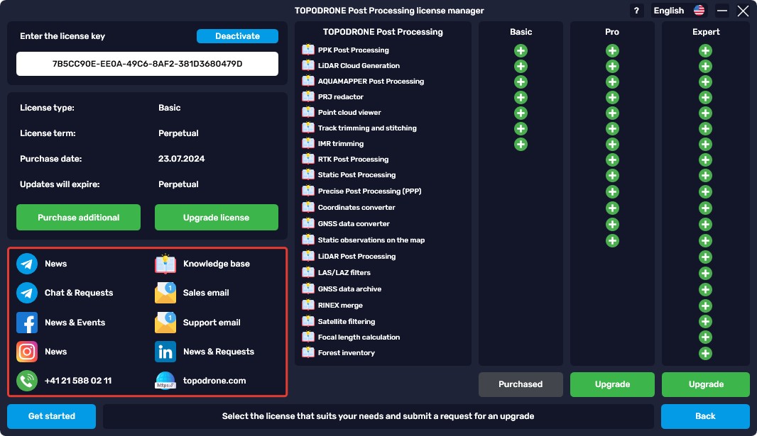
Feedback from TOPODRONE is available through all specified communication channels to resolve any issues that arise.
Starting the program and entering the key
Program Initialization: When you start the software, the bootloader window opens, where the user can start the installation and activation process.
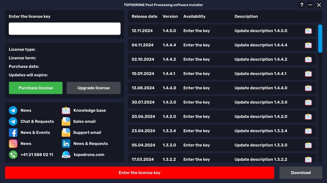
Entering the license key: If you have a valid license key, you must enter it in the designated field marked "Enter the license key".
The license key consists of 36 characters and has the format: ********-****-****-****-************. If your key consists of 19 characters and is presented in the form ****-****-****-****, this indicates that it belongs to the previous licensing system and is not suitable for current versions of the software. To get a new license key, it is recommended to use the "Support Mail" button or send a request to the email address support@topodrone.com, specifying the name of the equipment used and the name of your organization.
Display of available versions: After successfully entering the license key, information about available software versions will appear in the right part of the program interface. Versions that are available for download and installation within the current license key validity period are highlighted in blue, while gray indicates versions that require a license renewal to be used.
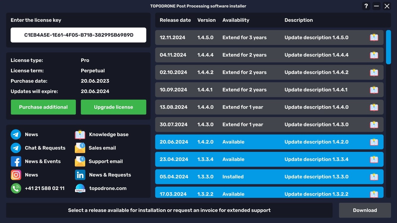
Software Update: To update the TOPODRONE Post Processing software, select the appropriate line in the list of available versions, which will be highlighted in green, then click the "Download" button and specify the folder path to save the downloaded file.
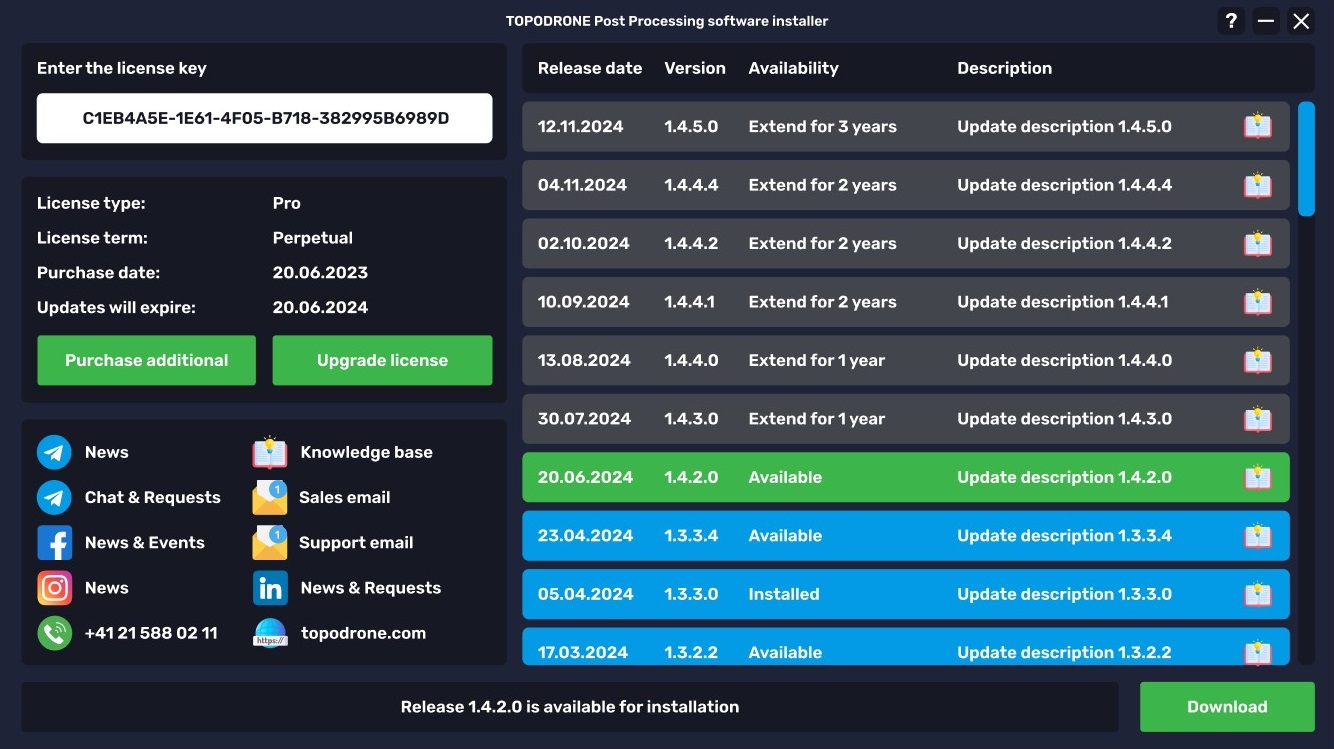
Displaying the download progress: The download progress percentage will be displayed at the bottom of the window, which allows the user to track the process.
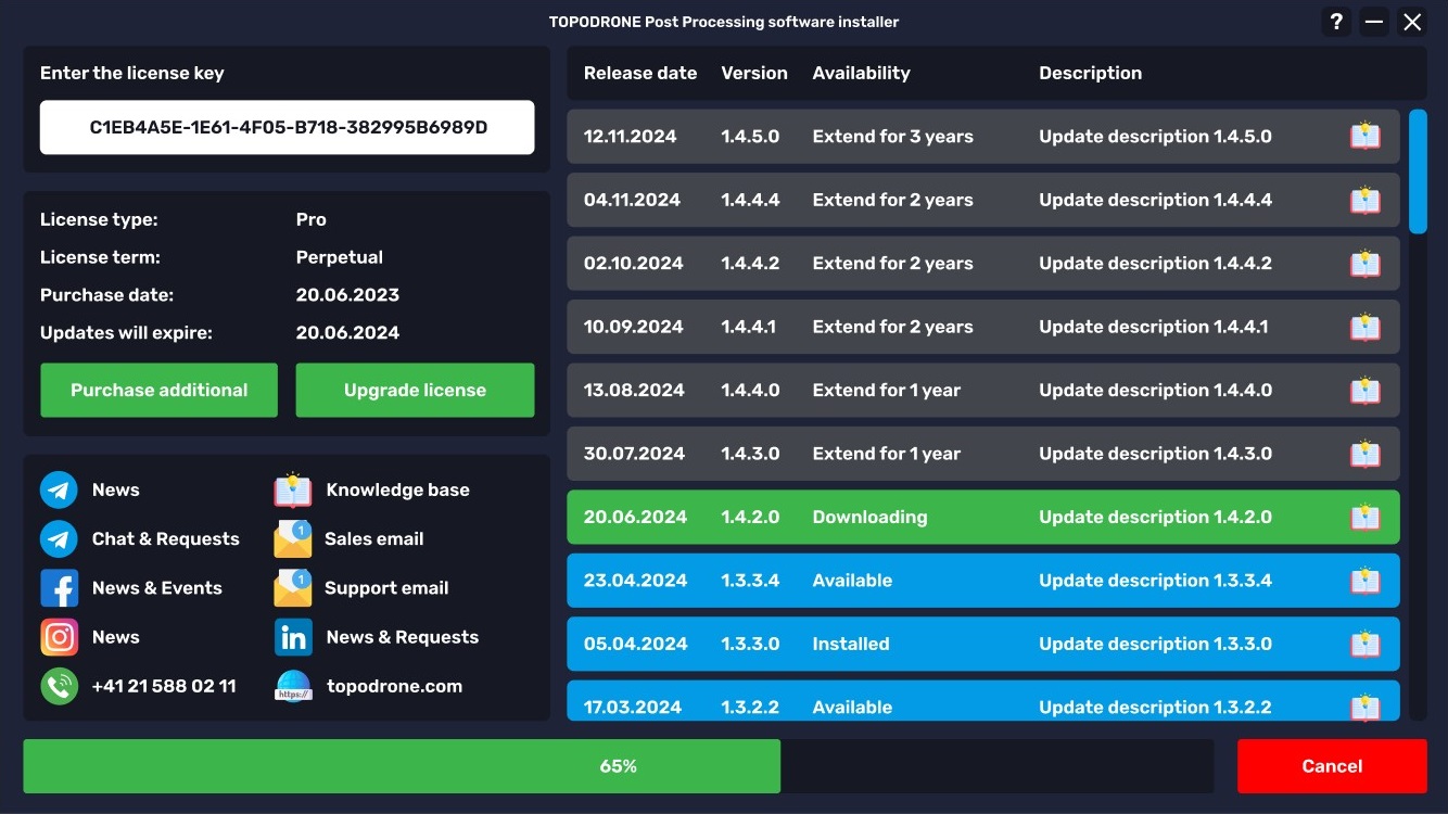
Installation Process: After the download is complete, the installer window will automatically open, where you must follow the standard procedures to complete the installation of TOPODRONE Post Processing software.
Activating the program: After successful installation, run TOPODRONE Post Processing. On the registration screen, enter your license key in the appropriate field for the serial number and click "Activate".
Ready to work: The program will be activated and ready for use, allowing you to successfully perform tasks related to post-processing data and implementing the functionality provided by the TOPODRONE system.
These steps provide a clear understanding of the software installation and activation process, making it much easier for users to interact with the product.
License renewal request
Software running w/o Internet connection
If there is no internet connection, the TPP software downloader will not be able to connect to the server. When you start the TPP software downloader, the following window will open with “Server is unavailable or no network connection” at the bottom.
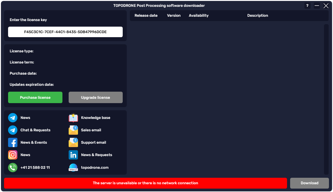
After connecting to the Internet, the TPP software downloader must be restarted.
Downloading installation files
Changes in licensing of the software "TOPODRONE Post Processing"
TOPODRONE announces significant changes to the licensing system for its TOPODRONE Post Processing software from 01.06.2023. As part of these changes, licenses will now be issued as activation keys, which will significantly simplify the process of obtaining and activating the software.
With the introduction of the new system, customers will no longer be required to use their personal account to activate the program. TOPODRONE Post Processing is now activated by entering the key in the appropriate field on the screen. This activation method makes the process more convenient for users, as it allows them to avoid additional steps related to account management.
However, successful activation of the software will still require access to the Internet. This is necessary to verify the validity of the entered key and to confirm the license, which ensures licensing compliance and protects the software from unauthorized use.
TOPODRONE is confident that these changes will not only improve the user experience, but will also make the activation process more intuitive and faster. We want users to be able to focus on their tasks, not the hassle of managing licenses. With the new activation system, TOPODRONE Post Processing will be easier to use and communication with the program will be more efficient.
Now all distributions are in TOPODRONE Software Distributor
TPP v.1.5.2.1 updated 27.07.2025
If the paid technical support period ended before 27.07.2025, then this distribution will not work for the user. He will need to either pay for support or download previous distributions, the release date of which is earlier than the paid support period ended.
Get the distribution: TOPODRONE Software Distributor
Added: Fixed bugs, improved security, accelerated operation, added new functionality compared to the previous version.
PPK Post Processing:
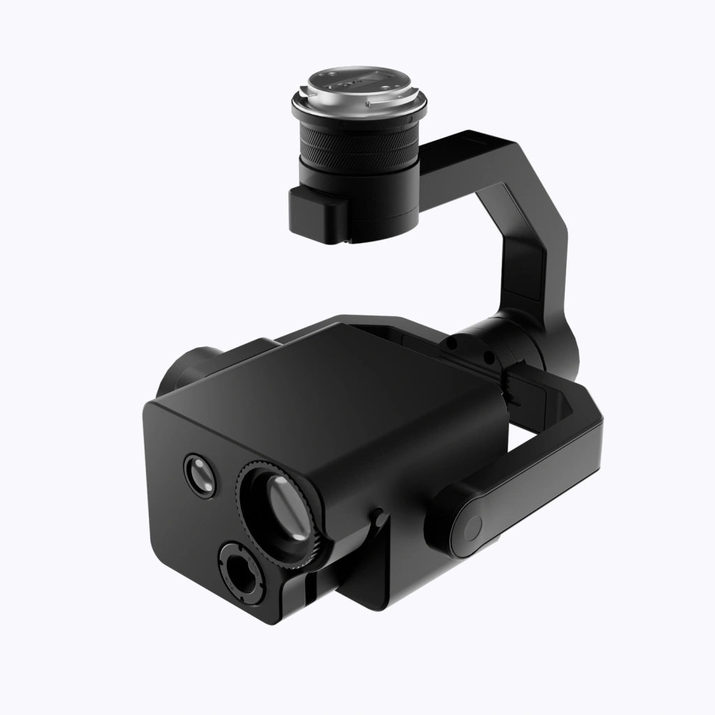
Added support for SWIR camera.
RTK Post Processing:
The photographic centers are adjusted to the offsets from the MRK file.
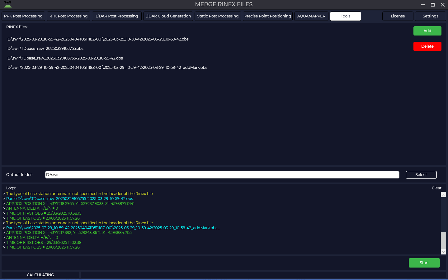
The utility "Merge RINEX files" is now available under the "PRO" license
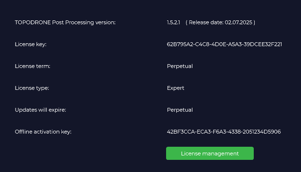
The release date can now be seen on the license information page:
Updated antenna file -> igs20_2353.atx
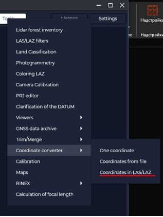
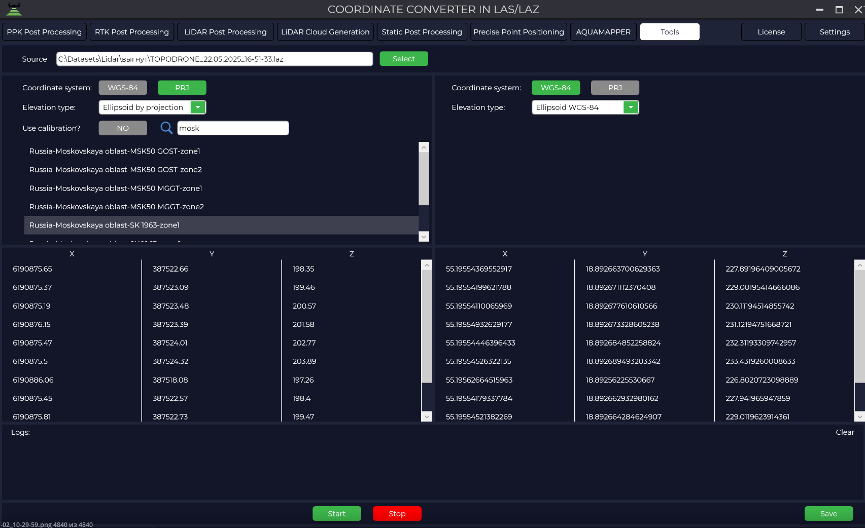
New utility for transforming point clouds from local/wgs84 to local/wgs84 coordinate systems:
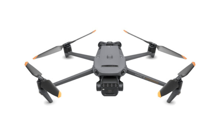
DJI Mavic 3 Multispectral Support:
PPK Post Processing/RTK Post Processing/LiDAR Post Processing:
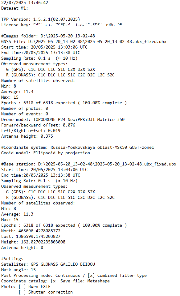
A log file is generated in the output folder for processing analysis or transfer to the technical support service.
PPK Post Processing/RTK Post Processing:
Accelerated display of markers on maps (photography center/GNSS marks/information).
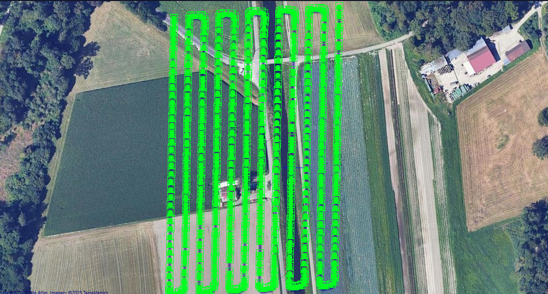
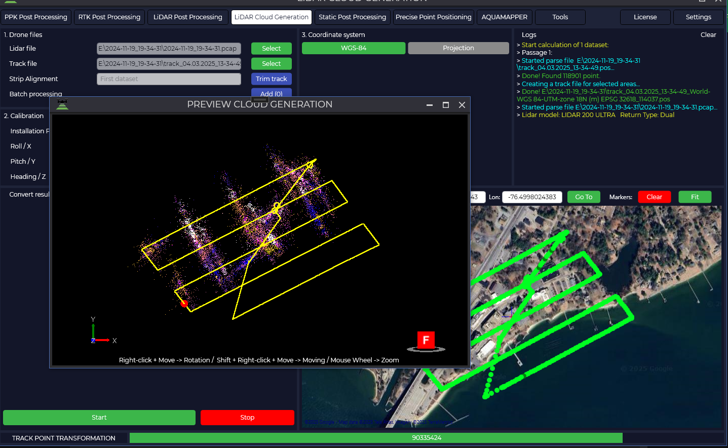
Lidar Cloud Generation:
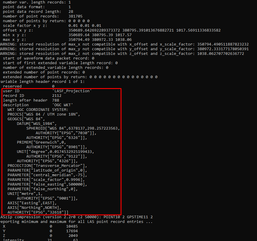
The calculation of calibration angles has been accelerated. Now the calculation time on the entire track or its part is performed equally in time. Calculated offsets are used for overflights. The lasinfo utility from the LAStools library has been integrated to check the correctness of LAS/LAZ headers. The PRJ information of the coordinate system in which the cloud is calculated is also added to the LAZ/LAS header.
Общее:
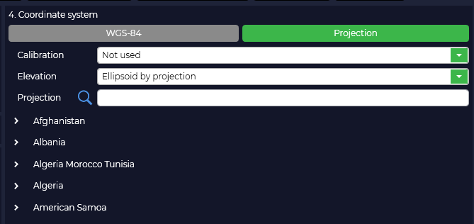
Speeded up loading of PRJ (about 6000 files) when starting the program.
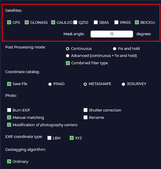
Added the ability to disable GPS grouping when calculating GNSS. Frequency trimming (L1/L2...) has been removed from the interface. All frequencies are included in the calculation.
TPP v.1.5.1.4 updated 07.03.2025
If the paid technical support period ended before 25.01.2025, then this distribution will not work for the user. He will need to either pay for support or download previous distributions, the release date of which is earlier than the paid support period ended.
Get the distribution: TOPODRONE Software Distributor
Added: Fixed bugs, improved security, accelerated operation, added new functionality compared to the previous version.
PPK Post Processing:
Added support for new UNICORE GNSS chips for all TOPODRONE models.
Added GNSS antenna offset presets for TOPODRONE P24 New + PPK + DJI Matrice 350.
Added automatic detection of typical offsets based on image tag data.
Implemented processing of data from TOPODRONE Q.FLY.
Antenna offset parameters are hidden from display
RTK Post Processing:
Implemented automatic loading of navigation files for each flight.
Fixed display of the "Plot" window in batch processing.
LiDAR Post Processing:
Fixed display of the "Plot" window in batch processing.
LiDAR Cloud Generation:
Added the ability to obtain point clouds along trajectories in local rectangular coordinates.
AQUMAPPER:
Improved automation of processes by implementing a filter for automatic removal of points with zero depth values.Added division of the TOPODRONE AQUAMAPPER Next dual-frequency sensor by frequencies in the *.LAZ format 200 kHz - 2 reflections, 450 kHz - 1 reflection.Added rounding of rectangular coordinates, heights and depths to three decimal places in *.CSV files.Reworked algorithm, allowing more accurate calculation of temperature for each measurement.
TPP v.1.5.1.3 updated 25.01.2025
If the paid technical support period ended before 25.01.2025, then this distribution will not work for the user. He will need to either pay for support or download previous distributions, the release date of which is earlier than the paid support period ended.
Get the distribution: TOPODRONE Software Distributor
Added: Bugs fixed, security improved, work accelerated, new functionality added in comparison with the previous version.
Fixed: LPP, PPK, RTK - The "Coordinate System", "Logs" and "Map" windows in the specified modules became the same size.
Fixed: RTK - When loading data into PPK Post Processing, the globe button for viewing the "Plot" window is not displayed, including during batch processing.
Added: LPP - Automatic check for missing IMU measurements with a trimming warning with the following text: "IMR file has time gaps, use the "IMR Trim" tool."
Added: PPK, RTK, LPP - Automatic check for rover and base station recording times. If the base station operating time does NOT include the rover operating time, then the message is displayed: "The base station operating time does not match the rover operating time.", if the base station operating time includes the rover operating time, then standard processing is performed. In the case of batch processing, all rover files are checked with the base station file.
TPP v.1.5.1.2 updated 28.12.2024
If the paid technical support period ended before 12/28/2024, then this distribution will not work for the user. He will need to either pay for support or download previous distributions, the release date of which was earlier than the paid support period ended.
Get the distribution: TOPODRONE Software Distributor
Added: Bugs fixed, security improved, work accelerated, new functionality added in comparison with the previous version.
Added: License information window, with the ability to launch the license management manager from the TPP interface.
Added: AQUAMAPPER: Support for dual-frequency echo sounder (200 kHz + 450 kHz). The low-frequency signal has a greater penetration depth, but poor detail, and vice versa, the high-frequency signal is more susceptible to scattering in water, but provides higher clarity and detail. Using a dual-frequency echo sounder increases the depth of signal penetration and the ability to separate weak reflected signals to obtain greater detail.
Added: PPK: Automatically converts shutter response time to a single format, which avoids doubling of marks. Finds gaps in shutter response marks and adds them to the stream through approximation.
Fixed: RTK: Adjusted the parameters of the "Dynamic" function. Previously, some data sets could not be calculated correctly.
Added: Updated RTKlib library (j->k)
Added: LCG Calculation of calibration angles A new algorithm has been developed with the introduction of a multiplier depending on the speed of movement (Accelerating the time to find corrections).
Added: AQUAMAPPER displays the trajectory in the Plot window
TPP v.1.4.5.0 updated 12.11.2024
If the paid technical support period ended before 11.12.2024, then this distribution will not work for the user. He will need to either pay for support or download previous distributions, the release date of which is earlier than the paid support period ended.
Get the distribution: TOPODRONE Software Distributor
+ Fixed bugs, improved security, increased speed and accuracy of calculations compared to the previous version.
+ Added: Support for GNSS receivers from Unicore (PPK module).

+ Fixed: In the RTK module bin is correctly converted to obs and nav.
+ Fixed: Improved generation of georeferencing file for photogrammetry.
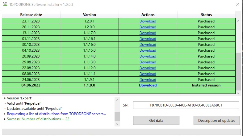
+ Added: The program is updated via the TOPODRONE distribution servers.
TPP v.1.4.4.4 updated 04.11.2024
If paid support expired before 04.11.2024, this TPP version will not work for a user. It is necessary to either pay for support or download previous version distributive, the release date of which is earlier than the expiration date of paid support.
Get the distribution: TOPODRONE Software Distributor
+ Fixed: correct conversion of *.bin to RINEX in RTK Post Processing module
+ Added: LiDAR Post Processing: Rinex.24O is converted to Rinex.obs before sending to IE.
+ Added: Camera calibration utility (Fix radial and tangential distortion in photos):
+ Added: PPK Post Processing module: additionally creates shutter time file (For LAZ coloring utility)
+ Added: LAZ coloring utility for photos
TPP v.1.4.4.2 updated 02.10.2024
If paid support expired before 02.10.2024, this TPP version will not work for a user. It is necessary to either pay for support or download previous version distributive, the release date of which is earlier than the expiration date of paid support.
Get the distribution: TOPODRONE Software Distributor
+ Fixed: AQUAMAPPER GNSS time has a day transition or batch post-processing of datasets taken over several weeks.
+ Fixed: SPP single vector/SPP network equalization/PPP: Updated links for downloading ephemeris from the server (University of California, San Diego [UCSD]), because NASA server does not have ephemeris for every day.
+ Fixed: LCG: During calculation of angles can make a large number of passes. Limit the number of passes = 10.
+ Added: “Clear logs” button in all modules.
+ Added: PRJ: Moved to the Server. Now they can be loades the same way as Geoids.
+ Fixed: PPK/RTK configuration files.
TPP v.1.4.4.1 updated 10.09.2024
If paid support expired before 10.09.2024, this TPP version will not work for a user. It is necessary to either pay for support or download previous version distributive, the release date of which is earlier than the expiration date of paid support.
Get the distribution: TOPODRONE Software Distributor
+ Added: when generating several clouds from the same trajectory, the trajectory is replaced in the Local Coordinate System (LSC). If 3 different clouds needs to be generated from one pcap file and from one trajectory after LiDAR Post Ptocessing module, TPP will generate 3 clouds and one trajectory for the last generated cloud. The trajectory in LSC have an additional prefix _CHMSS.
+ Fixed: during the LiDAR calibration angles calculation TPP can make a large number of passes. The algorithm for finding calibration angles is supplemented with automatic calculation of the scaling factor of the headings (depending on the velocity of motion). There should not be a large number of passes
+ Fixed: PPK/RTK modules: drone speeds in output catalogs are now taken from event.pos. Previously they were read from pos.stat, which in some situations were zeros.
+ Fixed: During processing of data from cameras without navigation centers of photos, after processing of trajectories the view was reset to coordinates 0;0. For all these cameras now the view on the screen does not change.
+ Added: LPP: it is now possible to enter the base station phase center coordinates in LSC, including taking into account the geoid model.
+ Added: AQUAMAPPER: In batch processing, simultaneous loading of UBX data is now available.
+ Fixed PPK: after TOPODRONE PT61 post-processing data if another data from any other camera that does not have a thermal imaging sensor post processing starts, a previews of the thermal imaging images are still generated.
+ Added: IMR Viewer: the vibration graph starts on 0
+ Fixed: Adjusted parsing of lidar file MID-360
TPP v.1.4.4.0 updated 13.08.2024
If paid support expired before 13.09.2024, this TOPODRONE Post Processing version will not work for a user. It is necessary to either pay for support or download previous version distributive, the release date of which is earlier than the expiration date of paid support.
Get the distribution: TOPODRONE Software Distributor
+ Fixed: Datum parameters refinement (we wrote our own code completely. Before third-party library used).
+ Fixed: Track stitching does not work correctly, the header is not correct.
+ Added: “Open catalog” button to calibration added.
+ Added: a “Slope Treatment” checkbox has been added to Land Classification.
+ Fixed: When exporting photo center catalog for Agisoft Metashape/3DSurvey, correct column formation is done.
+ Fixed: previews for thermal imager TOPODRONE PT61 were not generated correctly. There are different sensor sizes: 320 and 640 pixels.
+ Fixed: when the number of TOPODRONE PT61 photos and tags is different, the manual matching window does not exit and as a result the catalog of photo centers is not formed.
+ Added: the IMR viewer displays vibration graphs.
+ Fixed: the “Mark Time Correction” field in the photogrammetry settings returned.
TPP v.1.4.3.0 updated 30.07.2024
If paid support expired before 30.07.2024, this TOPODRONE Post Processing version will not work for a user. It is necessary to either pay for support or download previous version distributive, the release date of which is earlier than the expiration date of paid support.
Get the distribution: TOPODRONE Software Distributor
+ Added: processing settings of the AQUAMAPPER module are displayed in the UI. Added roll/pitch/bottom of water body infographics.
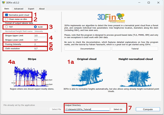
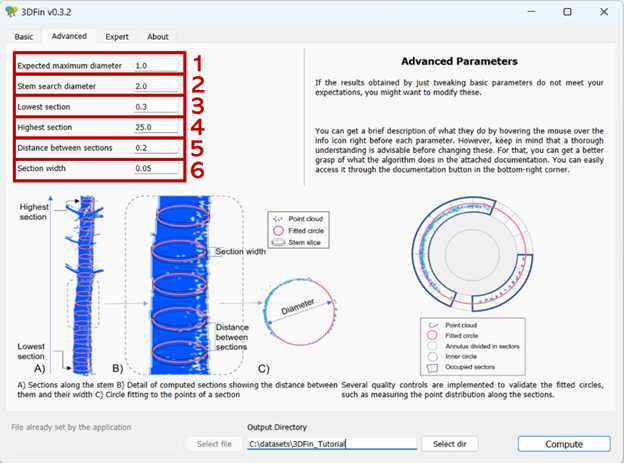
+ Added: forest inventory utility
TPP v.1.4.2.0 updated 20.06.2024
If paid support expired before 20.06.2024, this TOPODRONE Post Processing version will not work for a user. It is necessary to either pay for support or download previous version distributive, the release date of which is earlier than the expiration date of paid support.
Get the distribution: TOPODRONE Software Distributor
+ Added: multispectral + infrared camera support.
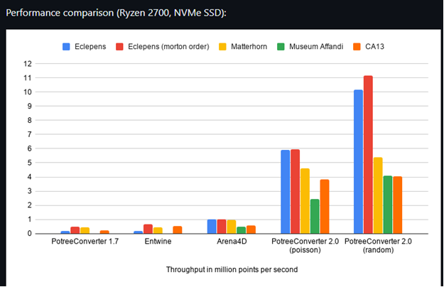
+ Updated: built-in viewer updated 1.7->2.1.
TPP v.1.3.3.4 updated 23.04.2024
If paid support expired before 23.04.2024, this TOPODRONE Post Processing version will not work for a user. It is necessary to either pay for support or download previous version distributive, the release date of which is earlier than the expiration date of paid support.
Get the distribution: TOPODRONE Software Distributor
+ Added: utility for trimming IMR file without GNSS. Used to trim an IMR file containing measurement omissions.

TPP v.1.3.3.0 updated 05.04.2024
If paid support expired before 05.04.2024, this TOPODRONE Post Processing version will not work for a user. It is necessary to either pay for support or download previous version distributive, the release date of which is earlier than the expiration date of paid support.
Get the distribution: TOPODRONE Software Distributor
+ Added: New algorithm for calculating calibration angles of lidar installation.
+ Fixed: length trimming works correctly for Hesai lidars.
+ Added: At group calculation of high-precision track 10 times less track points are displayed on maps (the program froze during rendering).
+ Added: In TopoSLAM, the return of the cloud to the track is accomplished by calibration.
TPP v.1.3.2.2 updated 17.03.2024
If paid support expired before 10.10.2024, this TOPODRONE Post Processing version will not work for a user. It is necessary to either pay for support or download previous version distributive, the release date of which is earlier than the expiration date of paid support.
Get the distribution: TOPODRONE Software Distributor
+ Added: AQAMAPPER module integrated
+ Added: LiDAR Calibration angles are now calculated and applied on a per-gal basis. It is used when specifying track inclination angles.
+ Added: WinPcap and .NET Core 3.1 Desktop Runtime are installed automatically.
TPP v.1.2.0.1 updated 23.11.2023
If paid support expired before 10.10.2024, this TOPODRONE Post Processing version will not work for a user. It is necessary to either pay for support or download previous version distributive, the release date of which is earlier than the expiration date of paid support.
Get the distribution: TOPODRONE Software Distributor
+ Added: switch in the settings to standard/expert modes. Expert mode allows the user to specify the IMU and lidar model. Standard mode performs automatic equipment detection.
TPP v.1.2.0.0 updated 20.11.2023
If paid support expired before 20.11.2023, this TOPODRONE Post Processing version will not work for a user. It is necessary to either pay for support or download previous version distributive, the release date of which is earlier than the expiration date of paid support.
Get the distribution: TOPODRONE Software Distributor
+ Added: Type of lidar survey is determined automatically (Aeral/Terrestrial)
+ Added: LiDAR firing direction is determined automatically (Forward/Backward)
+ Added: alternative calculation of track coordinates (algorithm of complex processing of GNSS angular positioning system information).
TPP v.1.1.17.0 updated 13.11.2023
If paid support expired before 13.11.2024, this TOPODRONE Post Processing version will not work for a user. It is necessary to either pay for support or download previous version distributive, the release date of which is earlier than the expiration date of paid support.
Get the distribution: TOPODRONE Software Distributor
+ Added: Static Post Processing: automatic addition of coordinates from GNSS files
+ Added: Lidar Cloud Generation: automatic UTM projection selection (if user has not specified a projection)
TPP v.1.1.16.1 updated 1.11.2023
If paid support expired before 01.11.2023, this TOPODRONE Post Processing version will not work for a user. It is necessary to either pay for support or download previous version distributive, the release date of which is earlier than the expiration date of paid support.
Get the distribution: TOPODRONE Software Distributor
+ Added: combined Kalman filter enabled by default, improves accuracy of GNSS calculations (in PPK/SPPP/PPP modules).
TPP v.1.1.16.0 updated 30.10.2023
If paid support expired before 10.10.2024, this TOPODRONE Post Processing version will not work for a user. It is necessary to either pay for support or download previous version distributive, the release date of which is earlier than the expiration date of paid support.
Get the distribution: TOPODRONE Software Distributor
+ Added: new algorithm for calibration angles calculation (used ICP for finding angles).
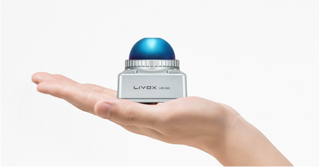
+ Added: MID-360 support
TPP v.1.1.15.0 updated 04.10.2023
If paid support expired before 04.10.2023, this TOPODRONE Post Processing version will not work for a user. It is necessary to either pay for support or download previous version distributive, the release date of which is earlier than the expiration date of paid support.
Get the distribution: TOPODRONE Software Distributor
+ Added: “Datum Refinement” utility
+ Updated: antenna directory for PPK, RTK modules
TPP v.1.1.14.0 updated 20.09.2023
If paid support expired before 20.09.2023, this TOPODRONE Post Processing version will not work for a user. It is necessary to either pay for support or download previous version distributive, the release date of which is earlier than the expiration date of paid support.
Get the distribution: TOPODRONE Software Distributor
+ Added: lidar rotation option relative to IMU (roll/pitch/heading)
+ Added: PRJ Editor utility allowing to correct PRJ parameters.
TPP v.1.1.13.0 updated 29.08.2023
If paid support expired before 29.08.2023, this TOPODRONE Post Processing version will not work for a user. It is necessary to either pay for support or download previous version distributive, the release date of which is earlier than the expiration date of paid support.
Get the distribution: TOPODRONE Software Distributor
+ Added: automated download of geoids from TOPODRONE server (199 geoids). Now geoids are not included in the distribution (reducing the size of the distribution), but are downloaded by users as needed.
+ Added: orthophoto generation module (Photogrammetry)
TPP v.1.1.12.0 updated 22.08.2023
If paid support expired before 22.08.2023, this TOPODRONE Post Processing version will not work for a user. It is necessary to either pay for support or download previous version distributive, the release date of which is earlier than the expiration date of paid support.
Get the distribution: TOPODRONE Software Distributor
+ Added: new version of high-precision track calculation with support for current TOPODRONE equipment is integrated
+ Added: filters for quality improvement: SOR and NOISE.
+ Updated: LAS/LAZ library (support for 1.3/1.4 formats)
+ Added: a utility to automatically “terrain” classify
TPP v.1.1.11.1 updated 08.08.2023
If paid support expired before 08.08.2023, this TOPODRONE Post Processing version will not work for a user. It is necessary to either pay for support or download previous version distributive, the release date of which is earlier than the expiration date of paid support.
Get the distribution: TOPODRONE Software Distributor
+ Added: HESAI lidars use calibration angles for installation
TPP v.1.1.9.1 updated 24.06.2023
If paid support expired before 24.06.2023, this TOPODRONE Post Processing version will not work for a user. It is necessary to either pay for support or download previous version distributive, the release date of which is earlier than the expiration date of paid support.
Get the distribution: TOPODRONE Software Distributor
+ Added: New PRJ filtering. Progressive full-text search is used. The search result is displayed line by line by full PRJ path.
TPP v.1.1.9.0 updated 04.06.2023
If paid support expired before 24.06.2023, this TOPODRONE Post Processing version will not work for a user. It is necessary to either pay for support or download previous version distributive, the release date of which is earlier than the expiration date of paid support.
Get the distribution: TOPODRONE Software Distributor
+ Added: Satellite filtering utility accelerated by 50 times
+ Added: A “ruler” for measuring distances has been added to all maps. You need to click twice on the map and the distance between these points will be written in the logs (in feet or meters depending on the “Feet” checkbox state).
+ Added: A new TOPOSLAM algorithm consisting of three stages has been added. At the first stage, the clouds are sequentially overlapped by generation time. The second stage is the mutual overlap of the clouds closest in distance. The third stage, using calibration, returns the position of the matched clouds to the track.
About
TOPODRONE Post Processing is a software, designed for processing RAW data acquired by TOPODRONE equipment. The application implements algorithms to perform trajectory calculation based on GNSS data, calculate high-precision coordinates of the image centers, joint processing of GNSS receiver and inertial system data, LiDAR point cloud generation and static data processing.
Convenience and universality of the interface allows the user to quickly master the TOPODRONE Post Processing. The software has three versions: Free, PRO and Expert.
Free - this version allows to calculate high-precision image centers acquired with TOPODRONE equipment, generate LiDAR point clouds (if you own a TOPODRONE LiDAR solution), process bathymetric data (if you own a TOPODRONE Aquamapper) and use various tools.
PRO - includes all the features of the Free version and adds the ability to calculate data using the PPP method and calculate accurate image centers from aircrafts equipped with a standard camera and RTK GNSS receiver.
Expert is the complete version of TOPODRONE Post Processing software and includes the whole complex of tools with joint processing of GNSS receiver and inertial system.
| Module |
Free | PRO | Expert |
| PPK Post Processing | + | + | + |
| RTK Post Processing | + | + | |
| LiDAR Post Processing | + | ||
| LiDAR Cloud Generation | + | + | + |
| Static Post Processing | + | + | |
| Precise Point Positioning | + | + | |
| AQUAMAPPER | + | + | + |
| TOOLS | + | + | + |
System Requirements
|
Minimal
Windows 10 or later (64 bit) Intel Core 2 Duo CPU 8 GB of RAM Dispaly resolution 1440×900 |
Recommended
Windows 10 or later (64 bit) |
Additional requirements: discrete graphics card, internet access to activate the software, mouse or other cursor control device, keyboard. For full installation of the program you need about 700 Mb on your hard disk.
Installation, activation and deactivation of the TOPODRONE Post Processing software
TOPODRONE Post Processing software can be downloaded from the official website of the developer https://topodrone.com/. To install it - run the *.exe file and follow the instructions. After successful installation, run the application. To change the language, press "Settings", then "General", select the necessary option and restart the software. Enter your serial number and click on the "Activate" button.
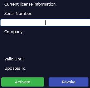
After successful activation, you will see the relevant information about the type of serial number, user Company name, software version, license validity period and the latest software update.
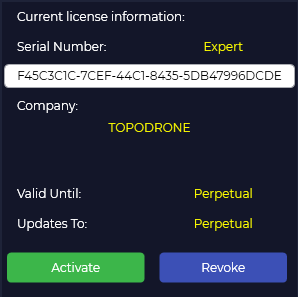
To deactivate the application on a current machine, click on the "Revoke" button. Only after this action you will be able to activate another device.
At the first run, you may get the following message: "To run this application, you must install .NET Core. Would you like to download it now?" It is necessary to download and install this library.
Preparation of initial data
After completion of the field works, prior to RAW data processing, it is necessary to organize the achieved dataset:
- Download the data to your computer. Photos from the camera and GNSS files from the PPK module of the aircraft; Data from the TOPODRONE LiDAR;
*.pcap – LiDAR sensor file
*.imr –file from the LiDAR IMU (Inertial Measurement Unit)
*.ubx – raw measurement file from the PPK Upgrade kit or built-in LiDAR PPK (GNSS) receiver
log.txt – LiDAR system log data, doesn't take part in processing stage, but necessary for diagnostics
*.raw – LiDAR system diagnostics data, not included in processing
*.ubx/.obs/.YYo/etc. - Static observation files from the base station;
Sample of the TOPODRONE LiDAR single dataset.
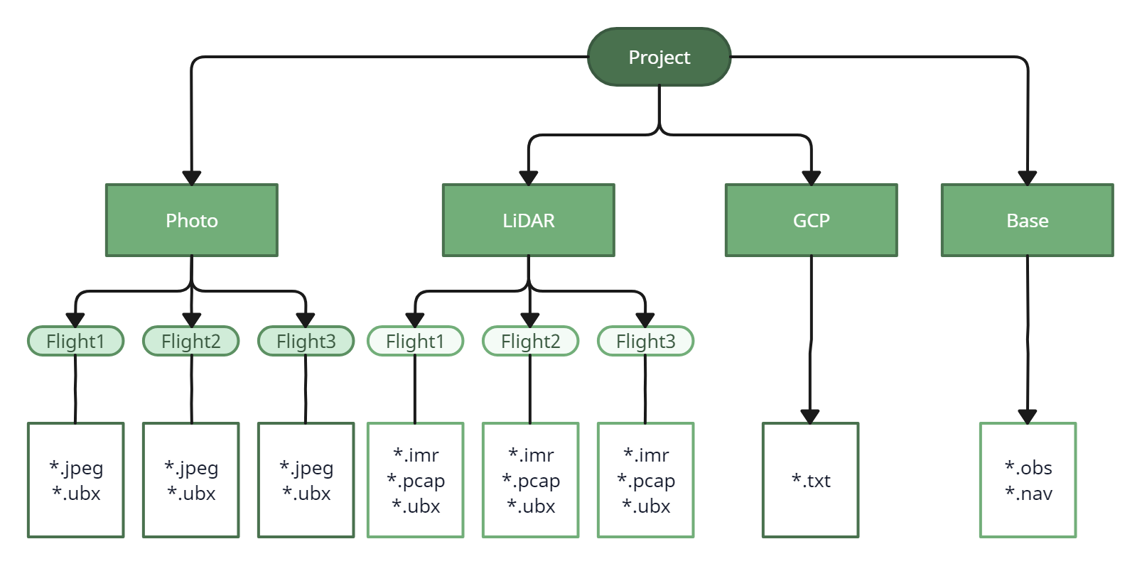
*.txt/.csv/etc. - Catalog of control point coordinates. - Distribute the data to a separate directories with an appropriate names. If you have had multiple flights and/or passes, each dataset shall be copied to a separate folder, accrodingly.
- Images dataset shall be separated according to the flights, as well as the *.ubx files from these flights, which are on a microSD flash card installed in TOPODRONE PPK Upgrade Kit on the aircraft.
Please note that the photos should be separated exactly by flight. In DJI aircraft, photos are named with a numerical designation from 1 to 999 (For example, DJI_0001.jpg and DJI_0999.jpg), if you have more than 1000 files, the system will start writing the images to a new folder named DJI_0001.jpg
- Be sure to convert the static observation file from the base station to RINEX format and move it to a separate folder, for example "Base".
|
|
| Example of data storage organization. |
PPK Post Processing
This module allows automatic processing of GNSS measurements, where a U-blox chip receiver acts as a rover. To perform processing in this module, perform the following procedure:
1. Run the TOPODRONE Post Processing.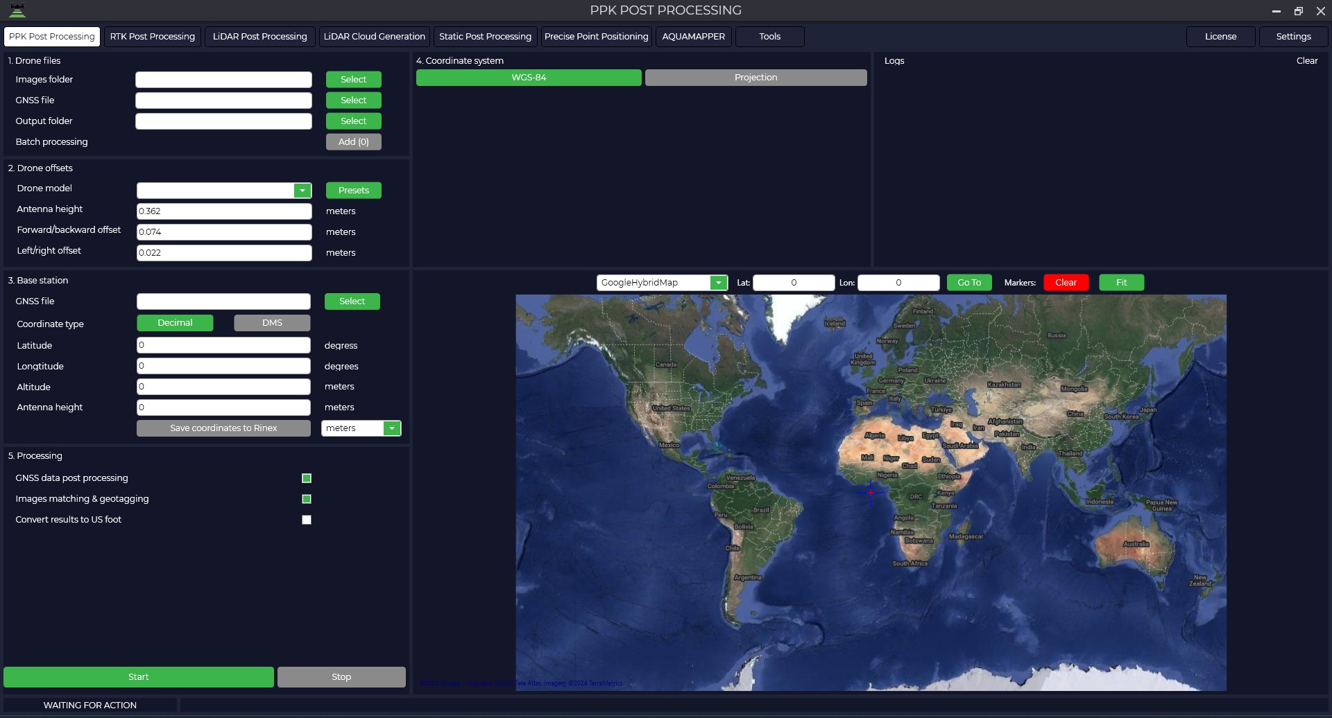
2. Select a folder with photos. The "Output folder" with final results of processing will be automatically created, if necessary it can be changed. If there is a *.ubx file from this flight in the folder with photos, data conversion to *.obs will take place. Otherwise it is necessary to select *.ubx file from this flight separately.
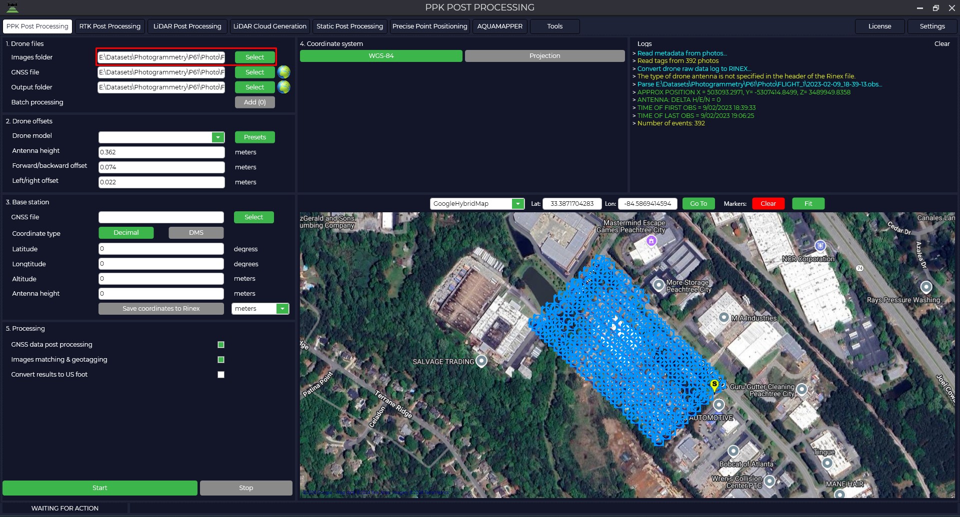
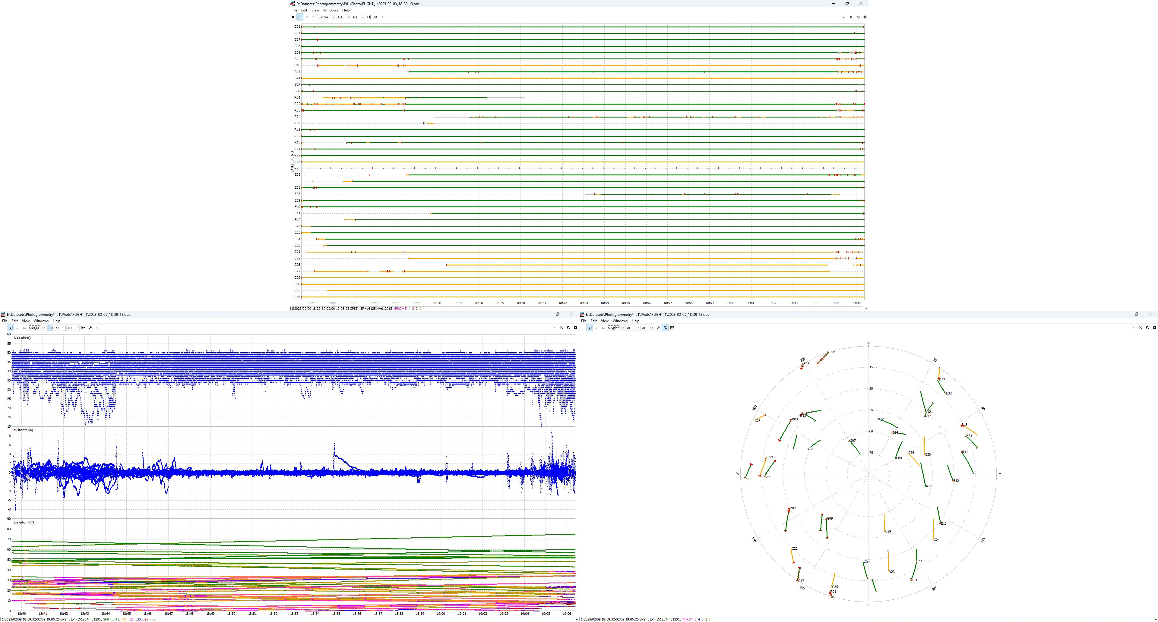
3. By pressing the button  you can analyze the quality of the data. For more information about data quality analysis, see Appendix B.
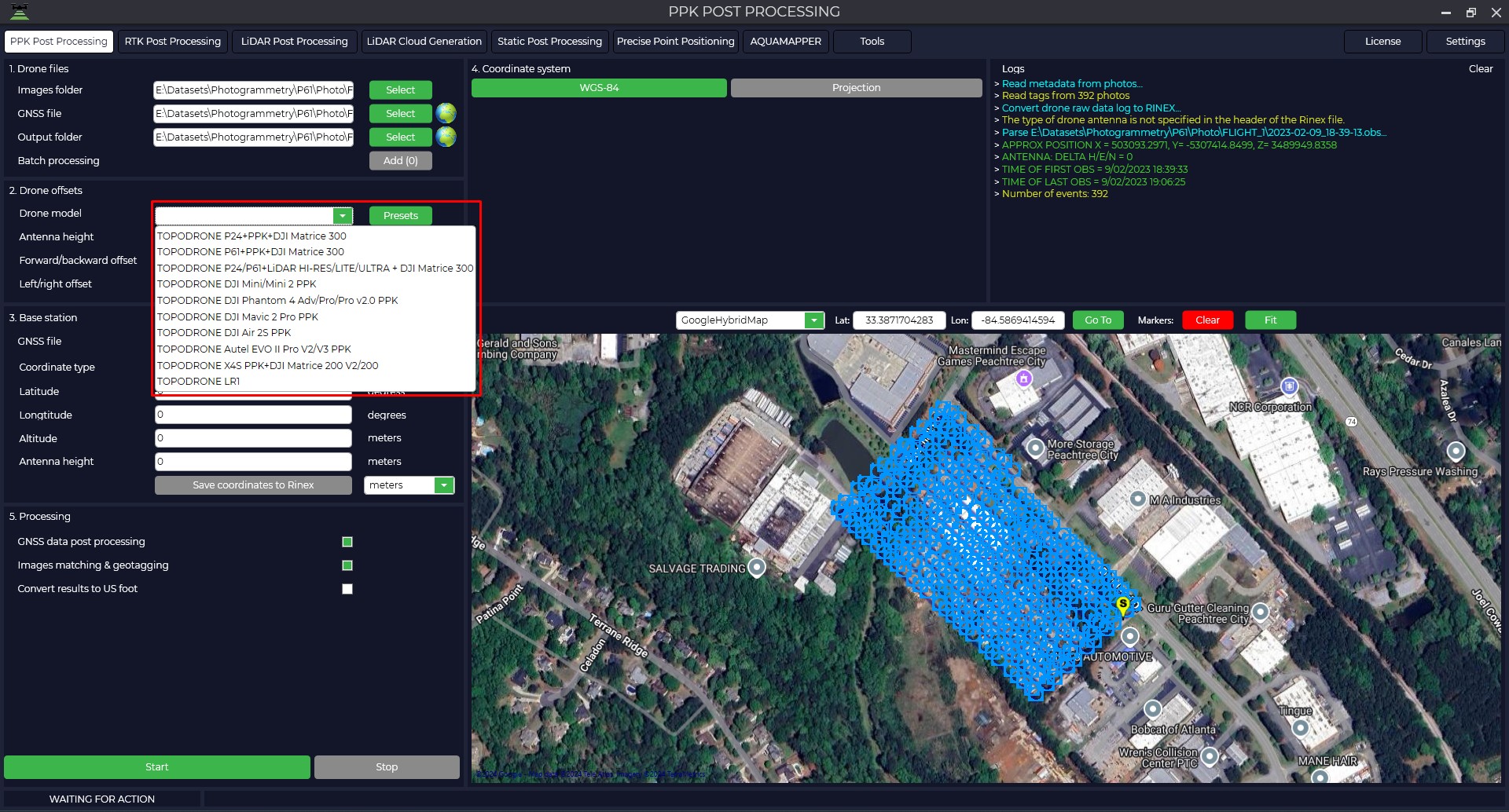
4. From the drop-down list select "Drone Model" to take into account the offset of the GNSS antenna and the center of the camera sensor. If necessary, you can add your own data to the drop-down list by clicking the "Presets" button and entering the necessary offsets.
5. Select the file from the base station (*.ubx, *.obs, *.rnx, *.YYo). For files in *.rnx and *.ubx formats, it will automatically start the conversion process to *.obs format
|
The "Logs" window displays information about actions performed by the program, it is necessary to pay attention to the time of file recording from the rover and from the base station. The base station file must overlap the rover files. |
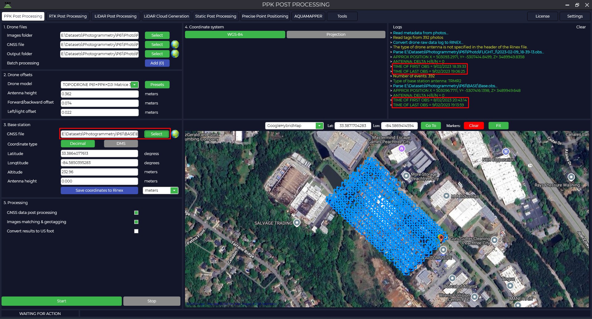
The TOPODRONE Post Processing will automatically load base station coordinates and base antenna height from the Rinex file, taking into account that it was entered during measurement
6. In case your coordinate system is different from WGS-84, you need to click the "Projection" button and select your coordinate system from the proposed list or enter the coordinate system name in the search bar.
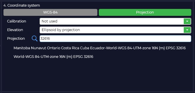
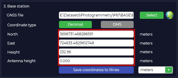
7. If your coordinate system is not in the list, you can add it to the TOPODRONE Post Processing program. When you select a coordinate system, it will be converted from WGS-84 to the selected projection. If necessary, correct the coordinates of the base station.
The height of the antenna includes the height of the milestone or tripod from the point of known coordinates to the bottom of the receiver mount and the height from the bottom of the receiver mount to the phase center.
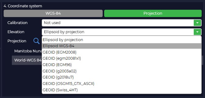
8. Change the type of height used, if you select any of the types, the height is automatically converted.
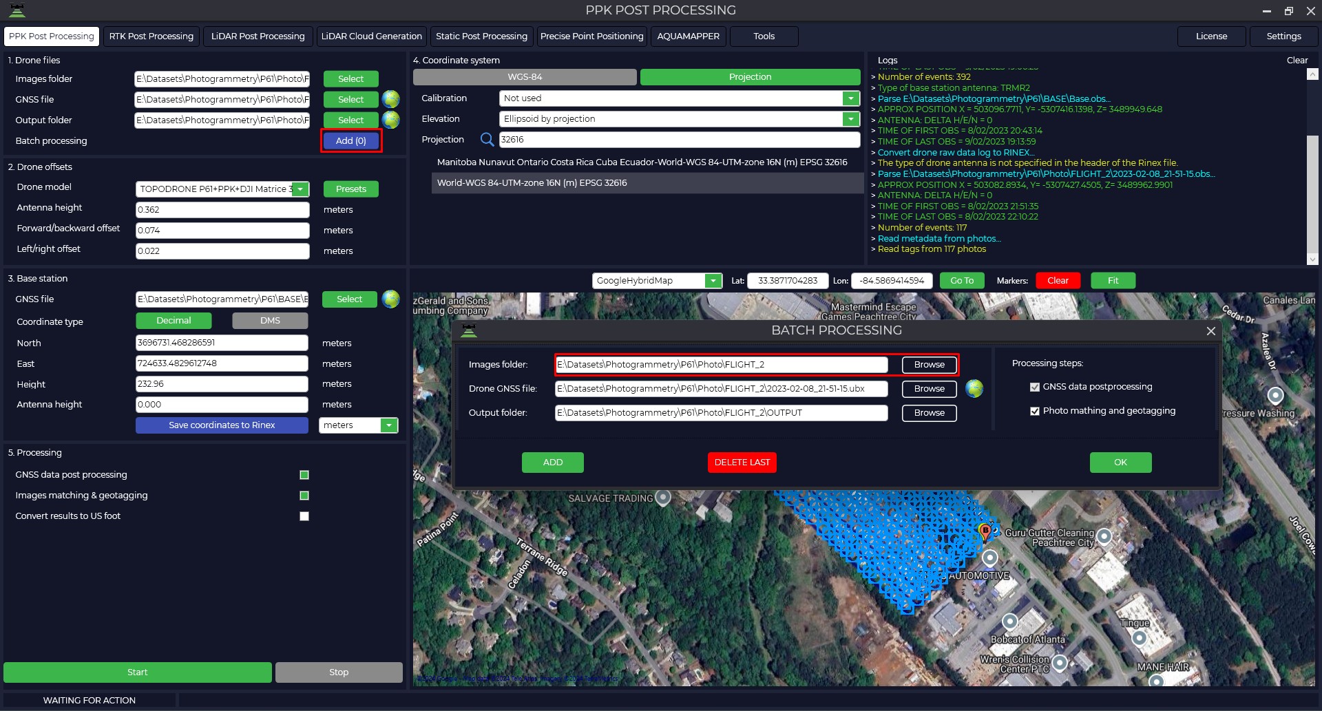
9. TOPODRONE Post Processing program allows to perform batch processing of many flights from one base station within one observation session. To start batch processing it is necessary to press the "Add (0)" button, in the opened window add additional folders with photos, *.ubx files and press "OK"
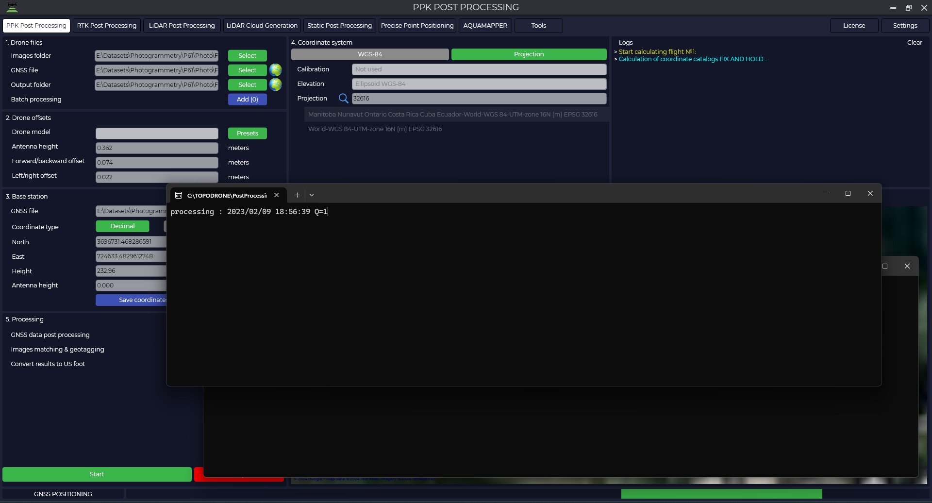
10. Just press the "Start" button to start the machining process. Data processing takes place simultaneously in forward and reverse directions and the type of solution is displayed in the form of the letter "Q" with the addition of a number, where Q1 - fixed solution, Q2 - floating solution and Q5 - no solution.
11. At the end of processing a window will be displayed, where you can see the trajectory of the rover, the number of photos, the number of marks, the number of matches and the accuracy of the obtained centers of photos, where green marks are marks obtained with a fixed solution, and yellow marks are marks obtained with a floating solution.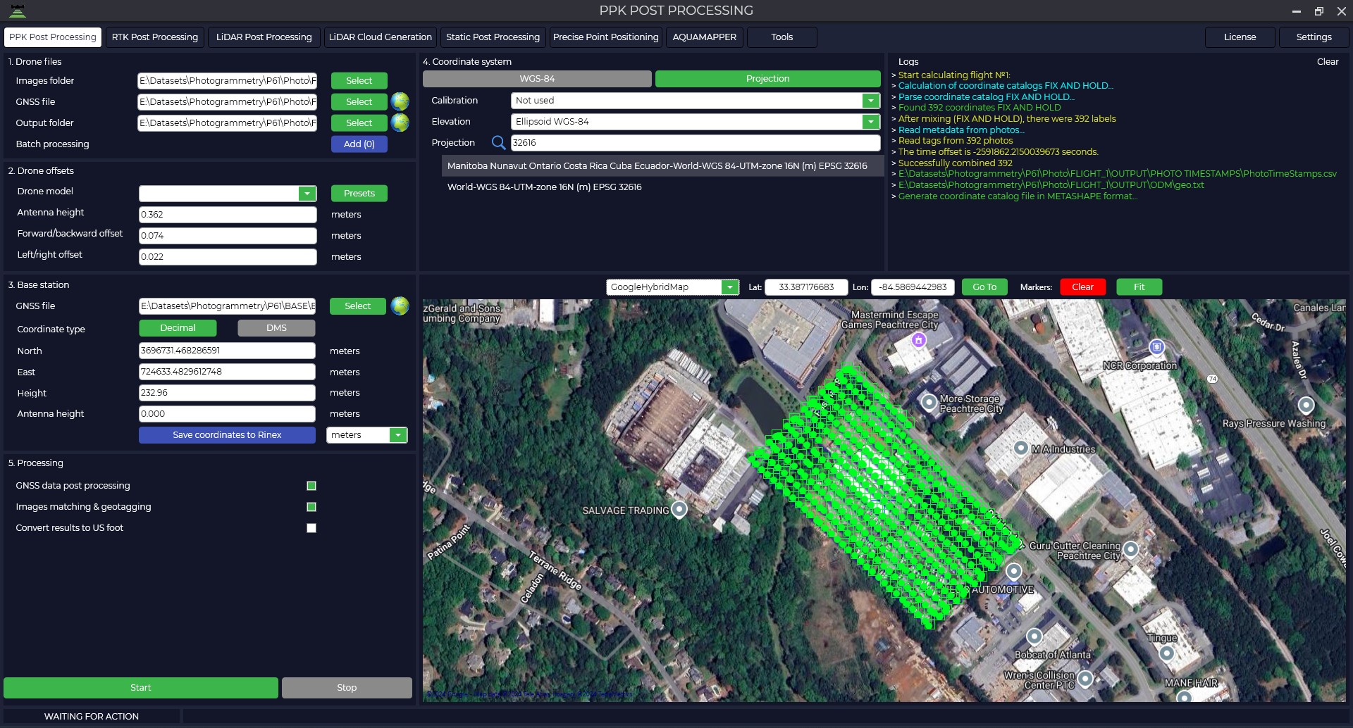
12. In the output folder, a catalog of coordinates of the exact photo centers is saved.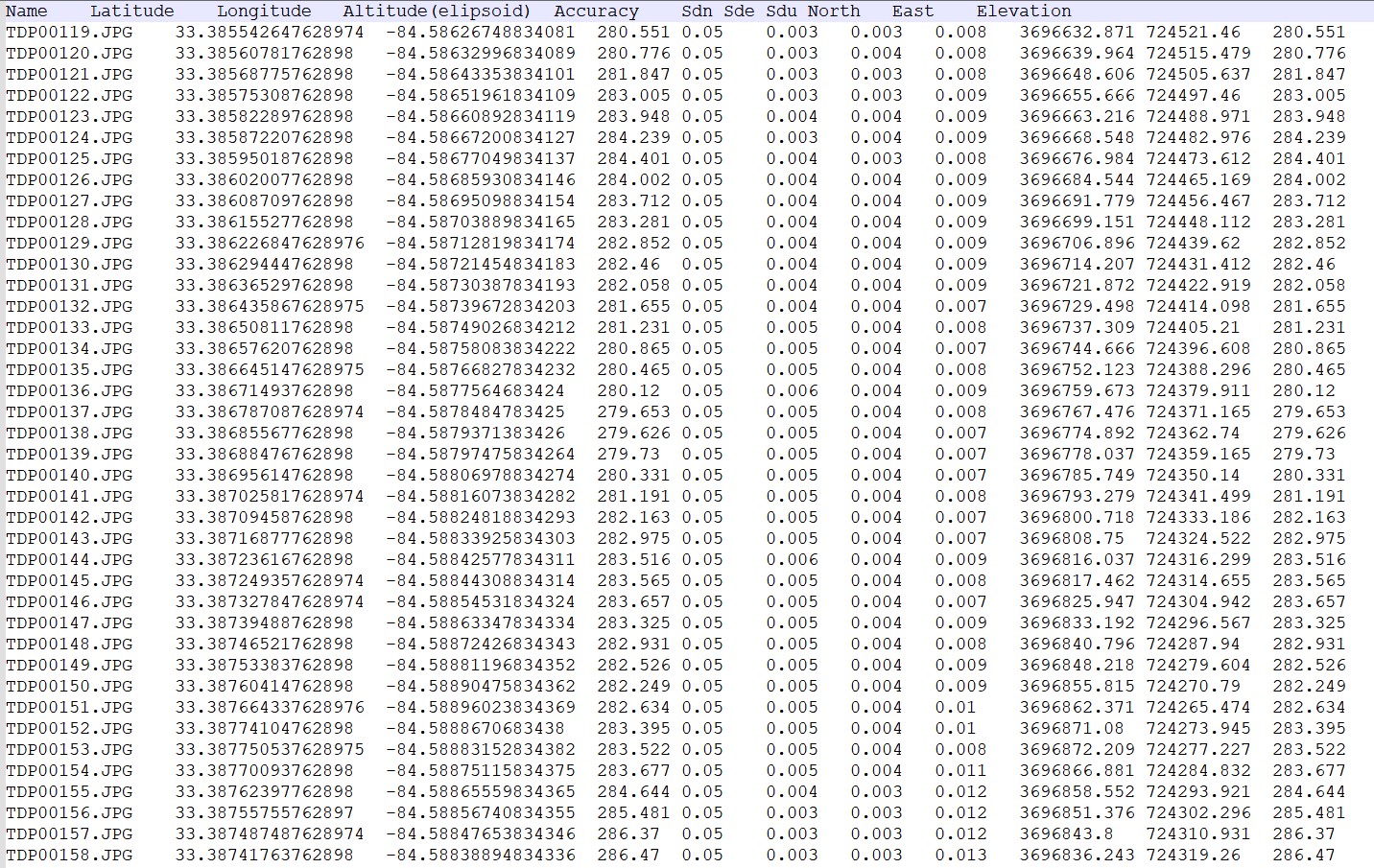
RTK Post Processing
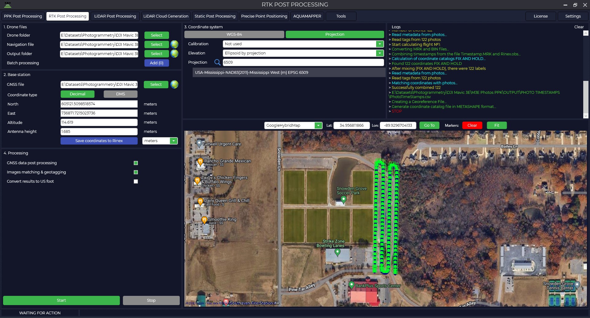
This module allows automatic processing of GNSS measurements from many aircraft, including DJI Phantom 4 RTK, DJI Matrice 300 RTK, DJI Mavic 3 Enterprise + RTK, Autel Evo II Dual RTK. To perform processing in this module, perform the following procedure:
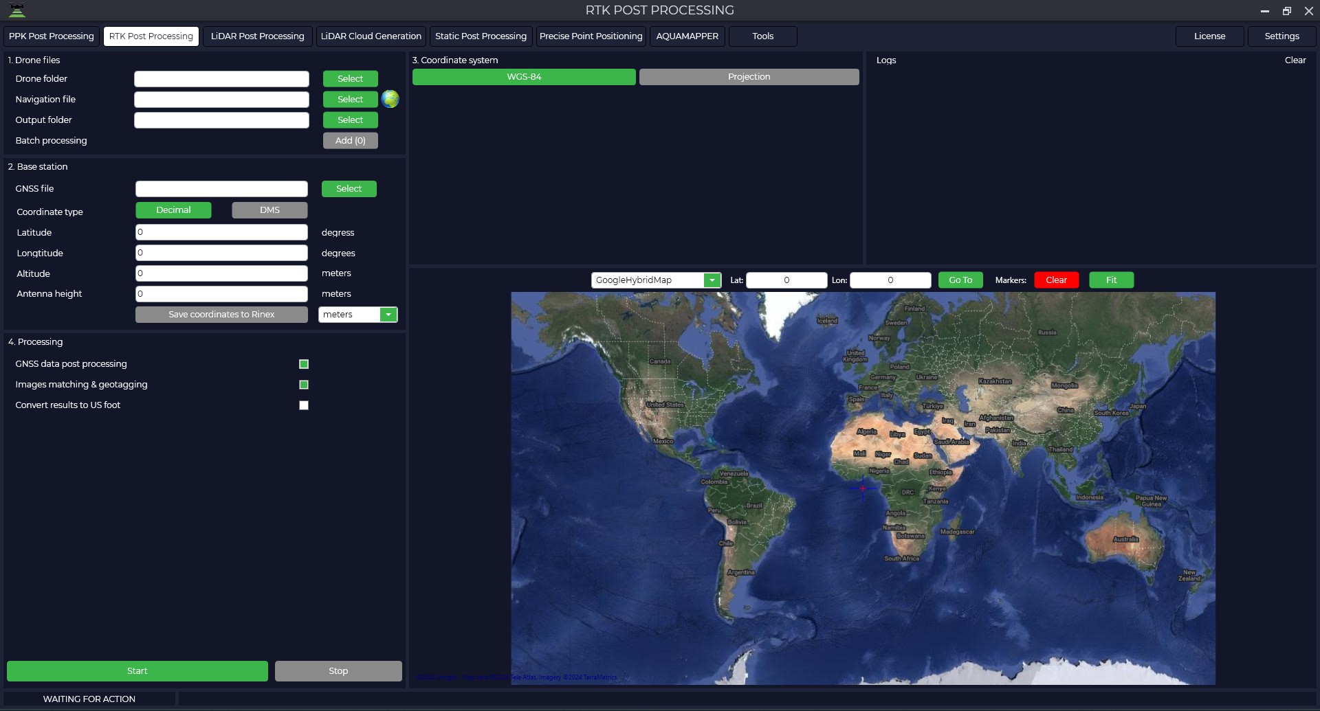
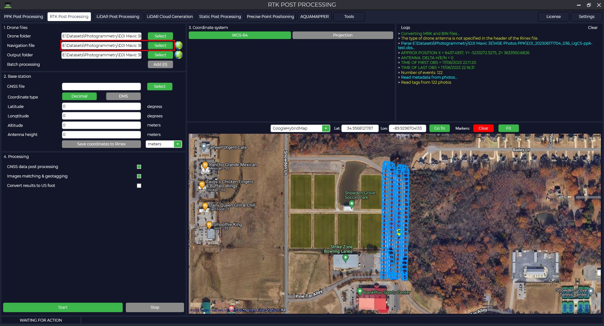
- Start the TOPODRONE Post Processing program and go to the tab RTK Post Processing.

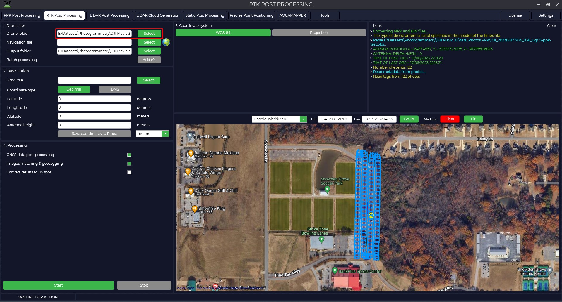
- Select the folder with the data collected during the flight. This folder should contain the following files: all photos without renaming or deleting, *.bin, *.obs, *.nav, and *.MRK. A folder with processed results will be automatically created, which can be modified if necessary.

- Select the *.nav file from the drone.

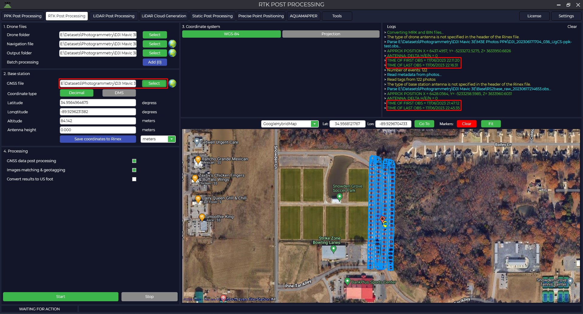
- Select the file from the base station (*.ubx, *.obs, *.rnx, *.o). For *.rnx and *.ubx files, it will automatically start the conversion process to *.obs format.
The "Logs" window displays information about actions performed by the program, it is necessary to pay attention to the time of file recording from the rover and from the base station. The base station file must overlap the rover files.

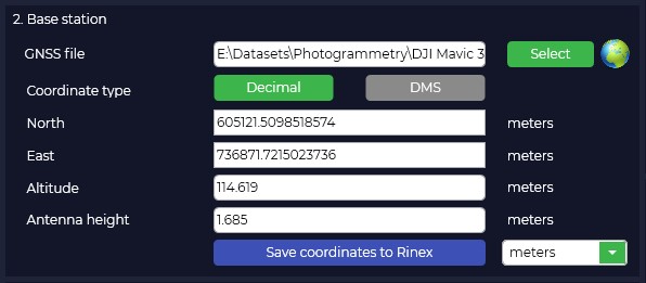
The program will automatically load base station coordinates and base antenna height from the Rinex file, taking into account that it was entered during measurement.
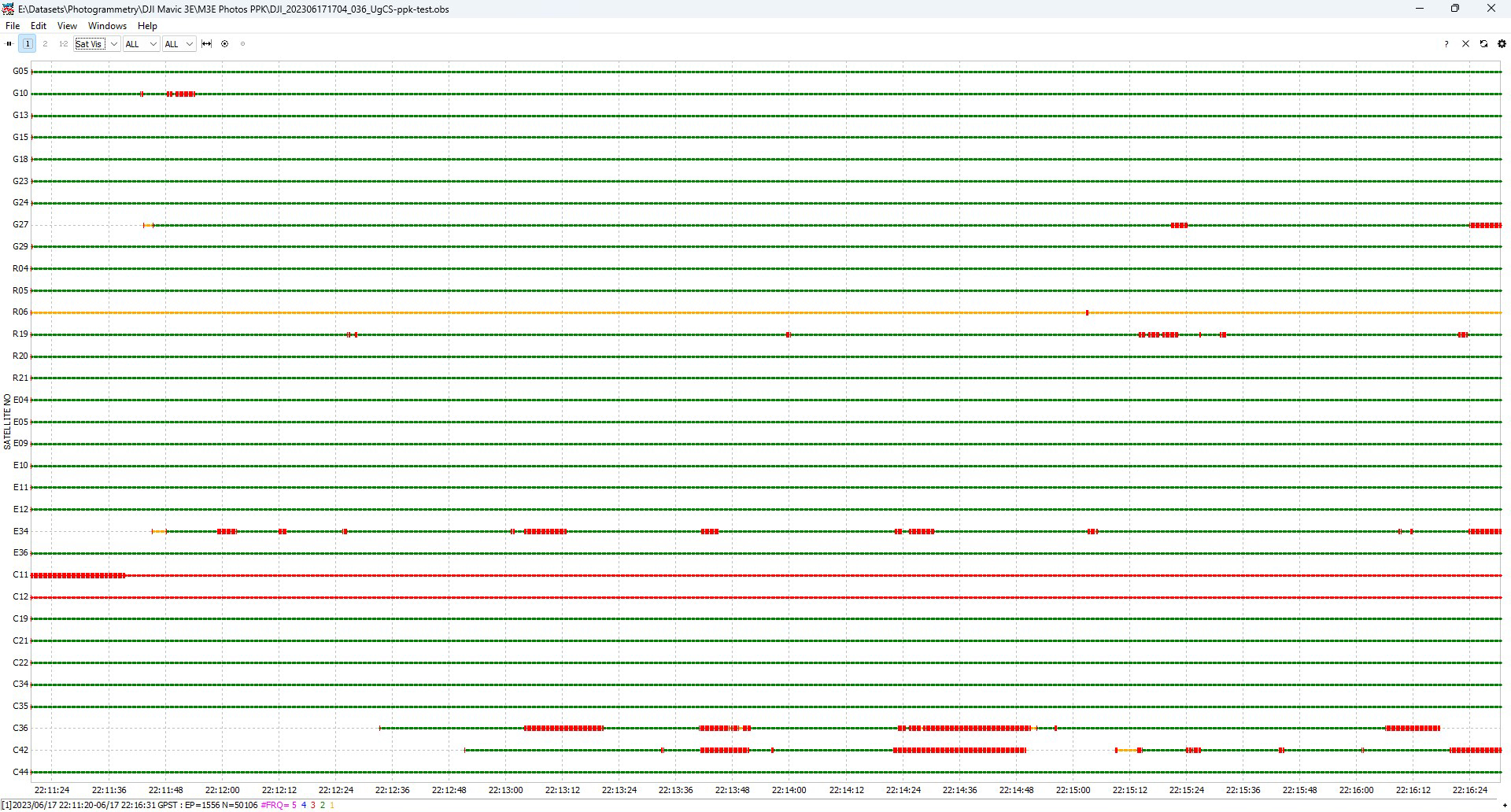
- By pressing the button you can analyze the quality of the data. For more information about data quality analysis, see Appendix B.

-
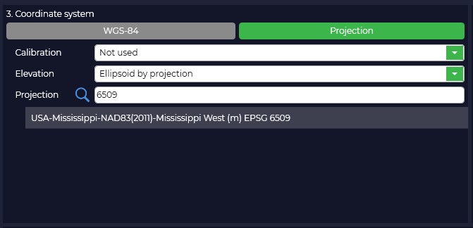
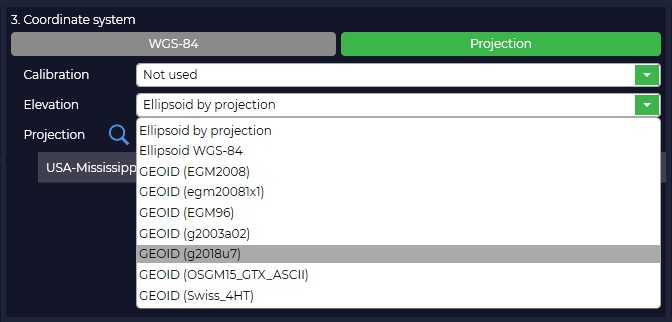
In case your coordinate system is different from WGS-84, you need to click the "Projection" button and select your coordinate system from the proposed list or enter the coordinate system name in the search bar. When you select the coordinate system, the conversion from WGS-84 to the selected projection will take place.

- If necessary, select the "Elevation Type" for your coordinate system.
If your coordinate system or geoid model is not in the list, you can add it to the TOPODRONE Post Processing program.
- If necessary, correct the coordinates of the base station.

Antenna height includes the height of the milestone or tripod from the point with known coordinates to the bottom of the receiver mount and the height from the bottom of the receiver mount to the phase center
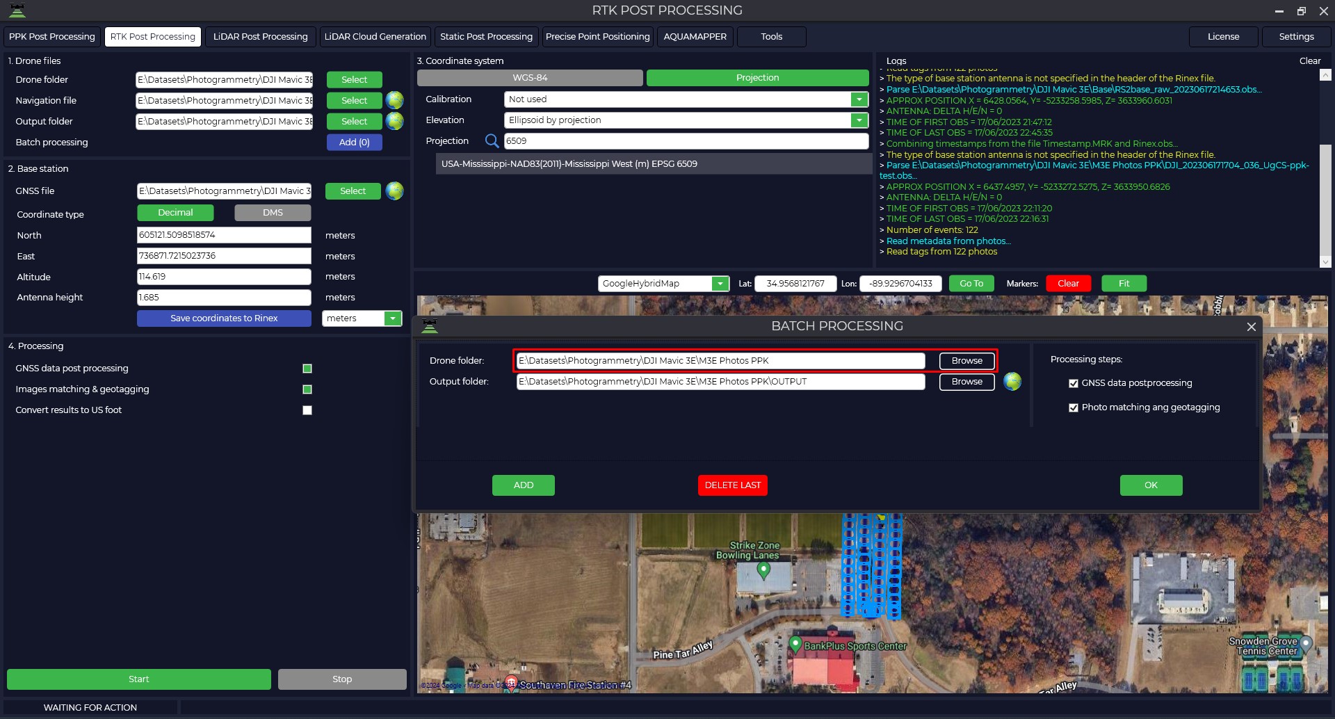
- TOPODRONE Post Processing program allows to perform batch processing of many flights from one base station within one observation session. To start batch processing it is necessary to press the "Add (0)" button, in the opened window add additional folders with other flights and press "OK"

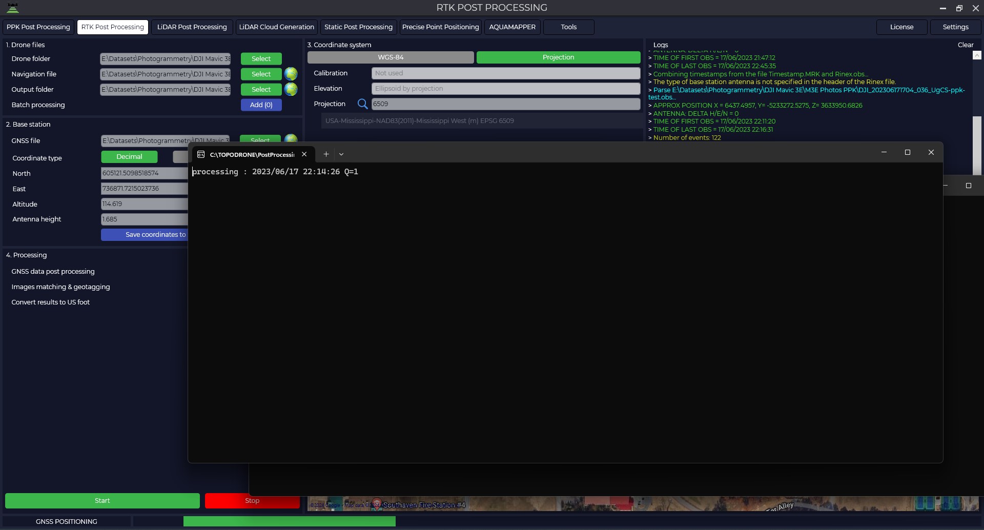
- To start the machining process, simply press the "Start" button. Data processing takes place simultaneously in forward and reverse directions and the type of solution is displayed in the form of the letter "Q" with the addition of a number, where Q1 - fixed solution, Q2 - floating solution and Q5 - no solution.

- At the end of processing a window will be displayed, where you can see the trajectory of the rover, the number of photos, the number of marks, the number of matches and the accuracy of the obtained centers of photos, where green marks are marks obtained with a fixed solution, and yellow marks are marks obtained with a floating solution.

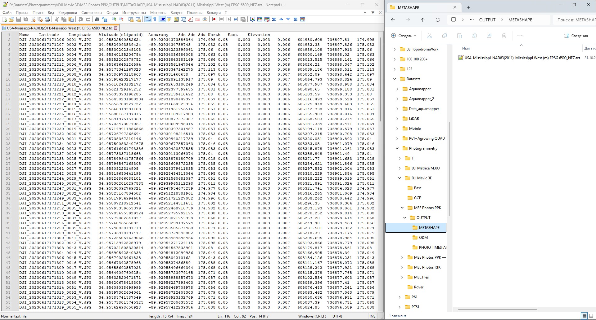
- The output folder stores a directory of coordinates of the exact centers of photography.

LiDAR Post Processing
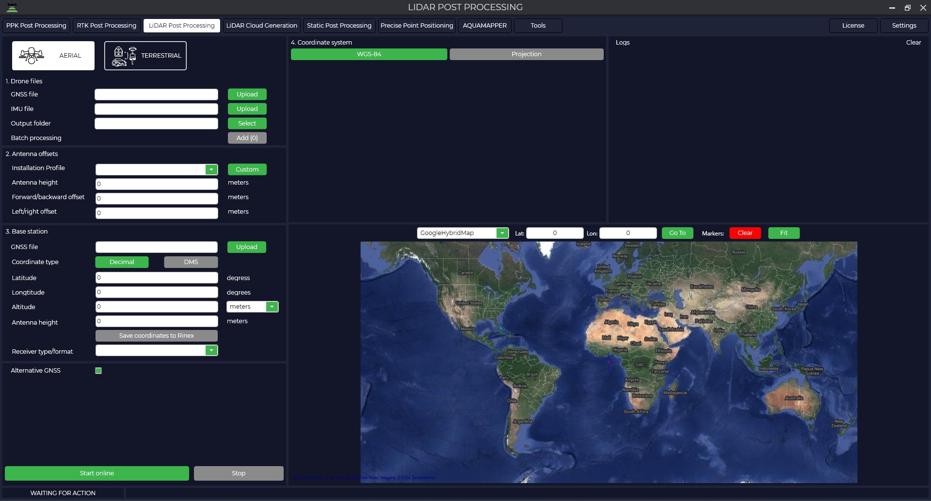
This module allows to calculate the trajectory of the laser scanner together with the inertial system data on the server solution of TOPODRONE company, thus not burdening the user's computer.
- In order to start processing it is necessary to start the TOPODRONE Post Processing program and go to the LiDAR Post Processing tab.

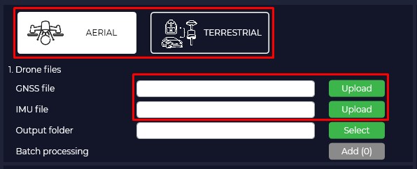
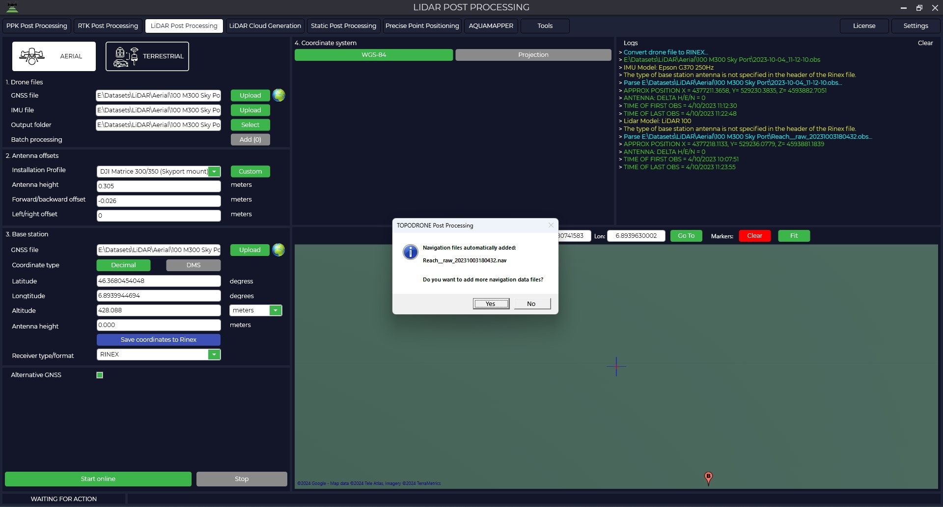
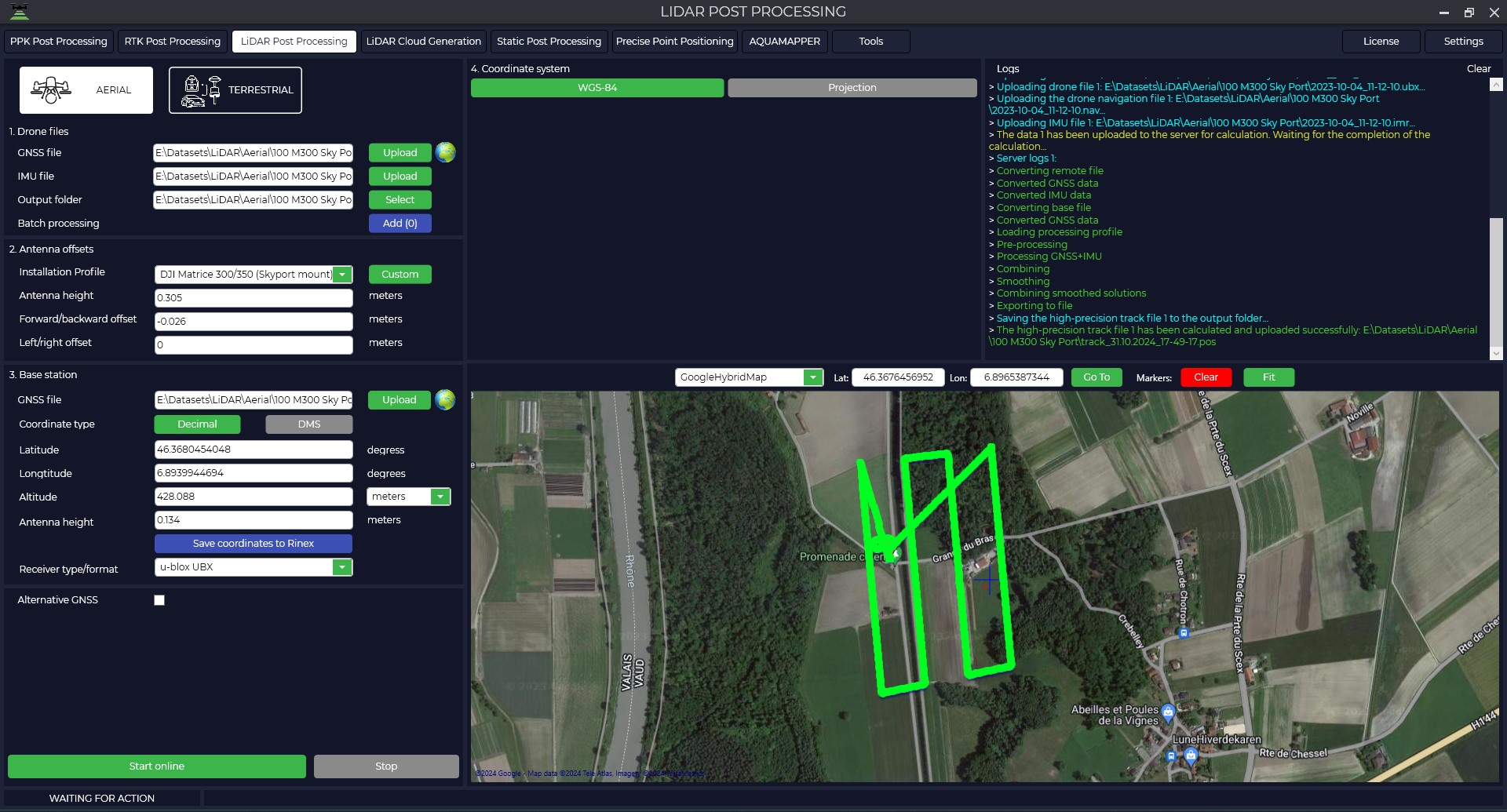
- Specify the installation type and path to the laser scanner files in the "GNSS file" field. Inertial data file will be loaded automatically in the "IMU file" field. Also by default the data will be saved to the source folder, but you can change the saving location in the "Output folder" field.

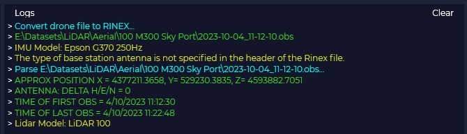
The "Logs" window displays all information on the downloaded files: type of scanner used, type of inertial system used, start/end time of file recording on the scanner and base station, as well as all information on data processing.

- By pressing the button you can analyze the quality of the data. For more information about data quality analysis, see Appendix B.

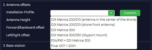
- Select your equipment model from the drop-down list.

The offsets will be loaded from the library automatically. Note that if you have selected the AERIAL setting type, the presets for TERRESTRIAL are not displayed.
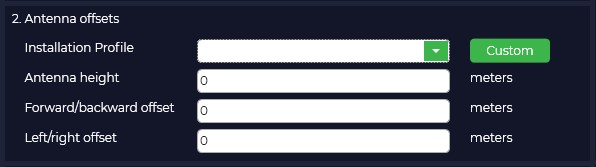
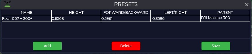
- If your offsets differ from the standard ones, you should click the "Add" button and enter your values.

-
If the IMU center is located behind, below and to the right of the GNSS antenna in the direction of travel, then at the post-processing stage the offset values are specified in TOPODRONE Post Processing software as positive values (without sign -) in meters. If the IMU center is located in front, above and to the left of the GNSS antenna in the course of movement, then at the post-processing stage the offset values are specified in TOPODRONE Post Processing software as negative values (with sign -) in meters. in meters.
The PARENT parameter is responsible for allowing the program to understand how the sensor was positioned during the scan. DJI Matrice 300 - sensor forward, P24/P61 + DJI Matrice 300 - sensor backward.

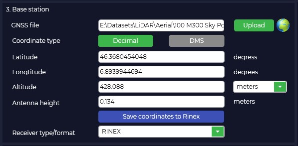
- Load the base station file in the "Base station" window in the "GNSS file" field.
When you download the measurement file of the base station in RINEX format, ephemeris will be automatically downloaded, you can download ephemeris from the TOPODRONE receiver that is installed in your laser scanner or downloaded separately.
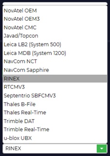
- From the drop-down list of receivers it is necessary to select the one that supports TOPODRONE Post Processing
TOPODRONE Post Processing program supports downloading data from different types of receivers, and if your receiver is not in the list, you can always convert the file to the universal RINEX format.

- Specify the high-precision coordinates of the base station.
Coordinates of the base station should be specified in the format latitude, longitude, height above the ellipsoid of the WGS 84 system.

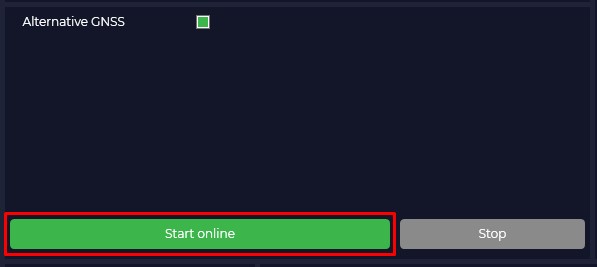
- Start processing by clicking the "Start Online" button.

Once processing starts, the data is uploaded to our server, where the trajectory is jointly processed using GNSS and IMU data. For correct processing you must have stable internet without interruptions, if there is a failure at the data upload stage, the processing stage will need to be restarted.
The "Alternative GNSS" checkbox allows you to get additionally the trajectory processed on your computer, possibly with a better solution quality.
-
At the end of processing the file with the high precision trajectory will be downloaded to your computer and in the map window you will be able to see the trajectory and the accuracy with which it was obtained. Green color means that the trajectory was processed with a fixed solution, yellow with a floating solution, and red color will tell us that with an offline solution. The trajectory file itself will be located in the default folder or in the folder you specified.

LiDAR Cloud Generation
To start this module, you need to go to the LiDAR Cloud Generation tab.
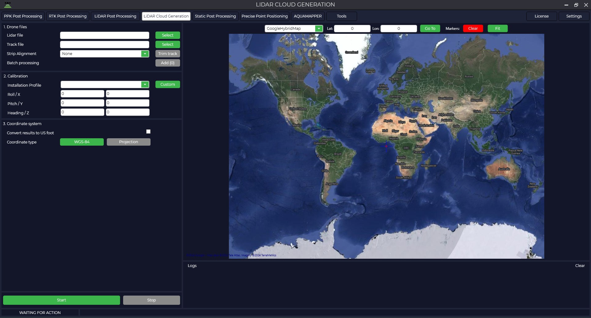
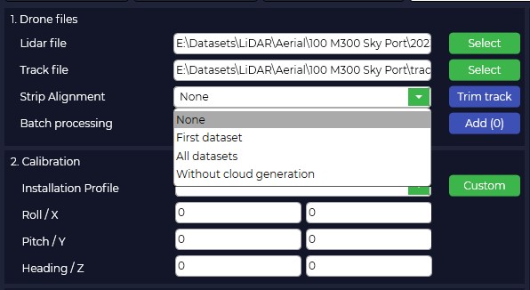
Specify the path to the data from the laser scanner *.pcap in the "Drone Files" window in the "Lidar File" field, in the "Track File" field specify the track_*.pos trajectory file, which was obtained as a result of processing in the LiDAR Post Processing module. By default, the data will be saved to the source folder.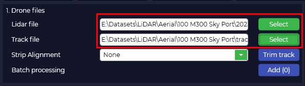
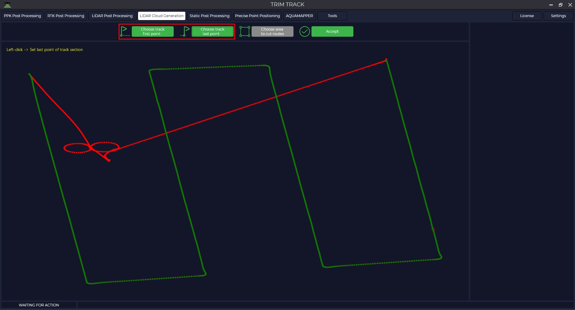
Click the "Trim" button and specify the start and end point of the trajectory to generate a point cloud.
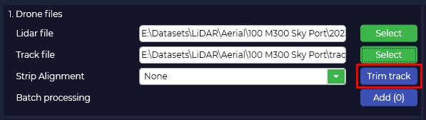
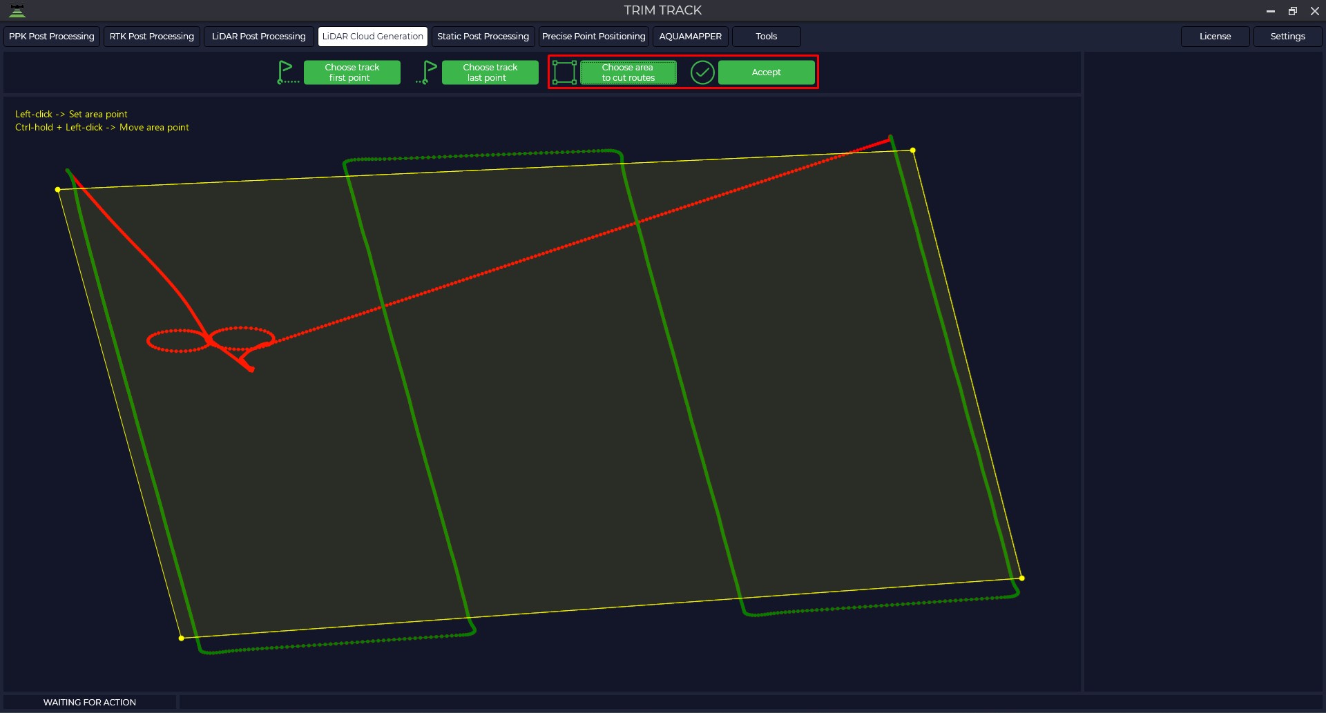
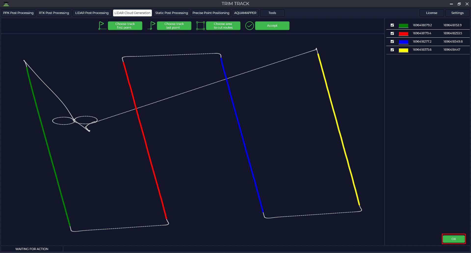
If necessary, you can divide the trajectory into separate transects by clicking on the "Trajectory trim area" button Click "Accept" to trim the unselected part of the trajectory and "OK" to save.
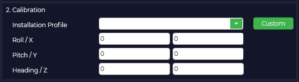
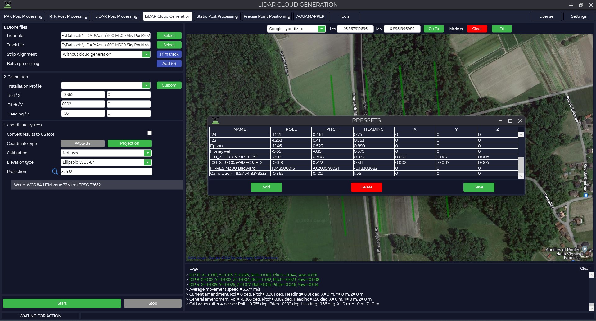
Roll, Pitch and Heading calibration angles should be set to "0", in case you have already calculated the angles and they remain stable, you can select your preset from the drop-down list. X/Y/Z should be used to correct the position of the clouds in the X, Y and Z axes in case of discrepancies between passes. Dynamics is the dynamic correction of Angle, Roll, Pitch and Heading across passes, i.e. each individual cloud segment will have its own angle values. If this function is used, the entire cloud must be used.
In the "Misalignment correction" field, you must select a value to calculate the angles. It is optimal to select at least two tack with a fixed trajectory with the presence of vertical objects.
To select a coordinate system you should press the "Coordinate system" button and choose your coordinate system from the proposed list or enter the name of the coordinate system in the search line. If your coordinate system is not in the list, you can add it to the TOPODRONE Post Processing program.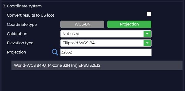
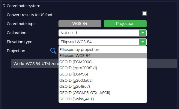
Change the type of elevation used. If your geoid model is not in the list, you can add it to the TOPODRONE Post Processing program yourself.
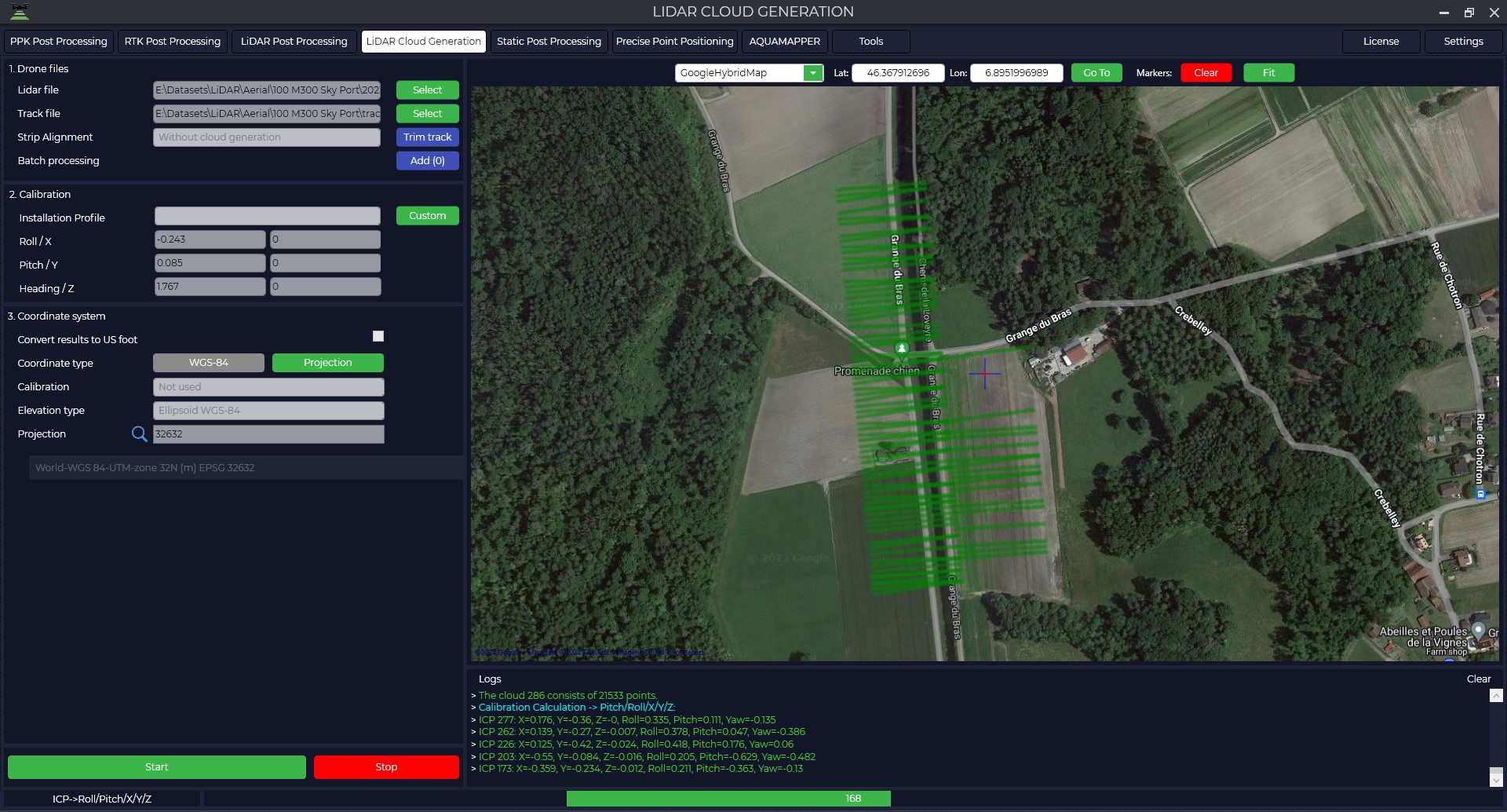
Next, click on the "Start" button to start the Angle Calculation or point cloud generation process.
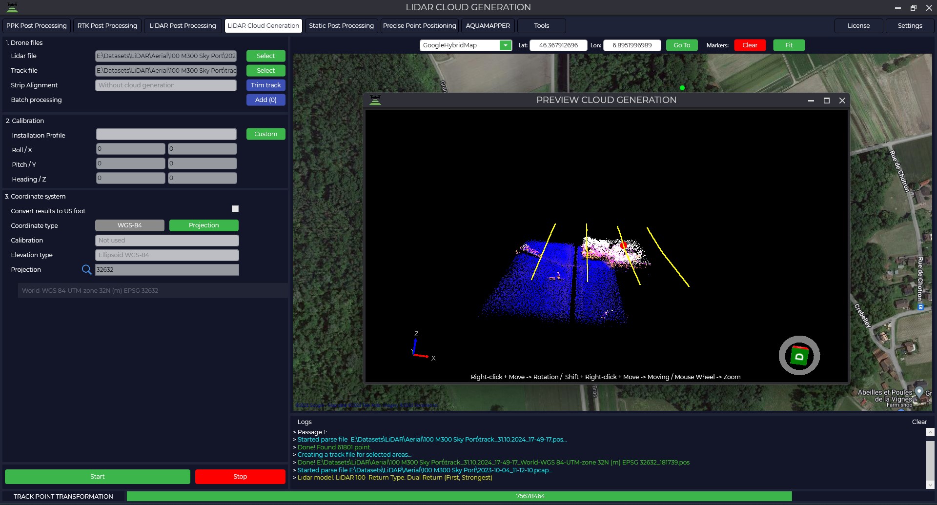
In the process of calculating the angles, the program will perform several passes, which will result in the calculated values of Roll, Pitch and Heading angles.
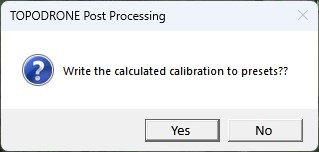
When the calculation is complete, the program will inform you that you can save the calculated calibration parameters into presets for further selection of values from the drop-down list.
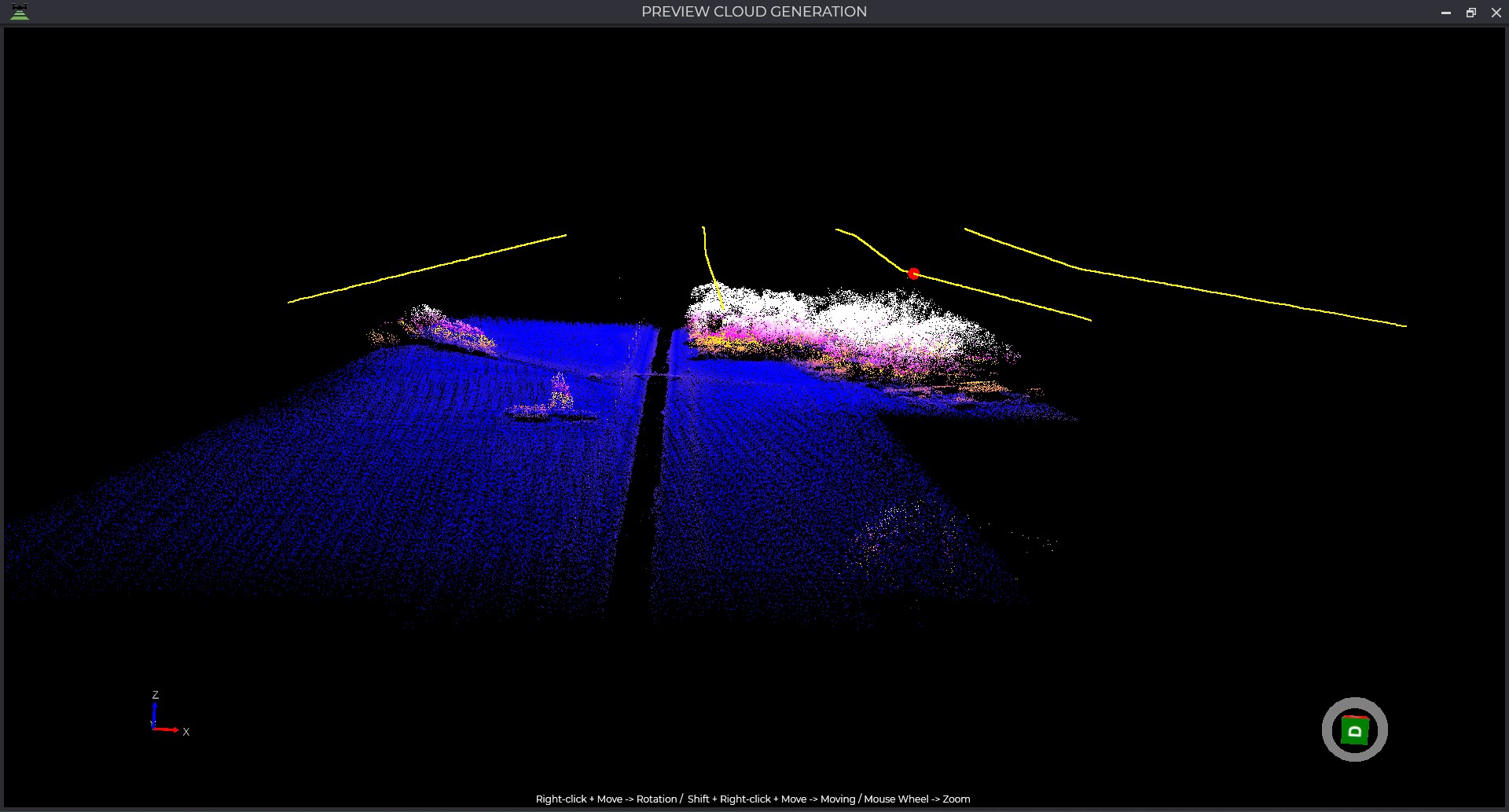
When completed, a cloud will be generated in LAS/LAZ format in the source data folder.
Static Post Processing
Module for processing GNSS data in static mode, consists of two parts:
- One vector
- Grid equalization
One vector calculates rover coordinates from base station by one vector. The measurement requires rover and base station files as well as a navigation file. Supported observation file formats: *.ubx, *.obs, *.rnx and *.*O.
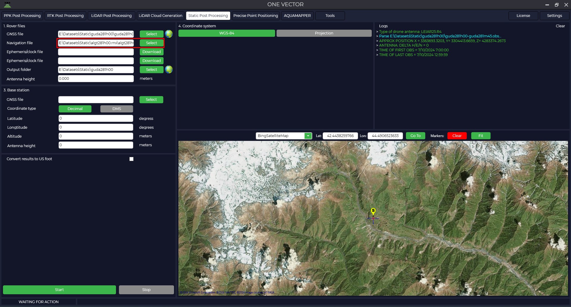
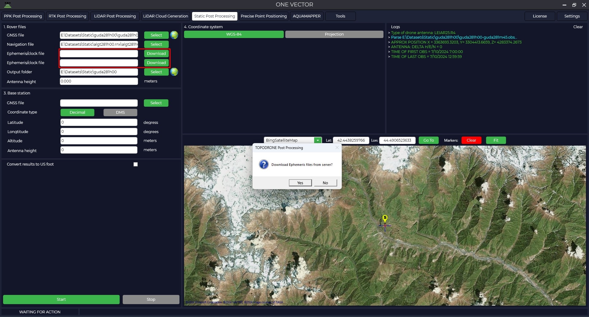
For more accurate results also upload your own or download an accurate ephemeris file from NASA server. Supported formats of navigation ephemeris files: *.nav, *.rnx, *.n, *.p, *.g, *.h, *.q, *.c and *.l. Supported formats of precision ephemeris files: *.eph, *.sp3.
The distance from the base station to the rover, using accurate ephemeris and NASA navigation file, is practically unlimited, daily rinex files give RMS of about 5 centimeters at a distance of 5 thousand km.
In the module it is possible to perform measurement in the selected projection at once.
One vector
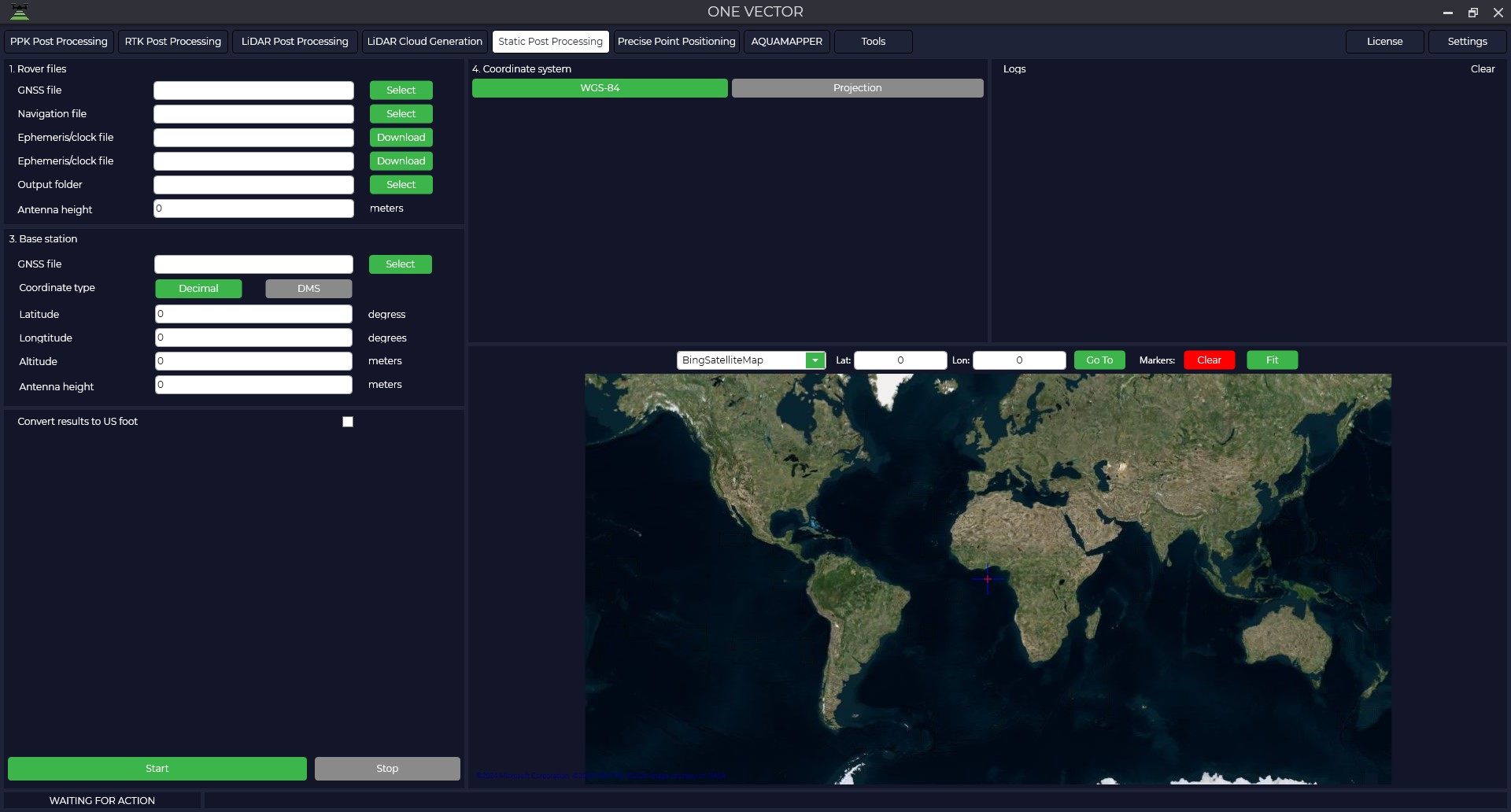
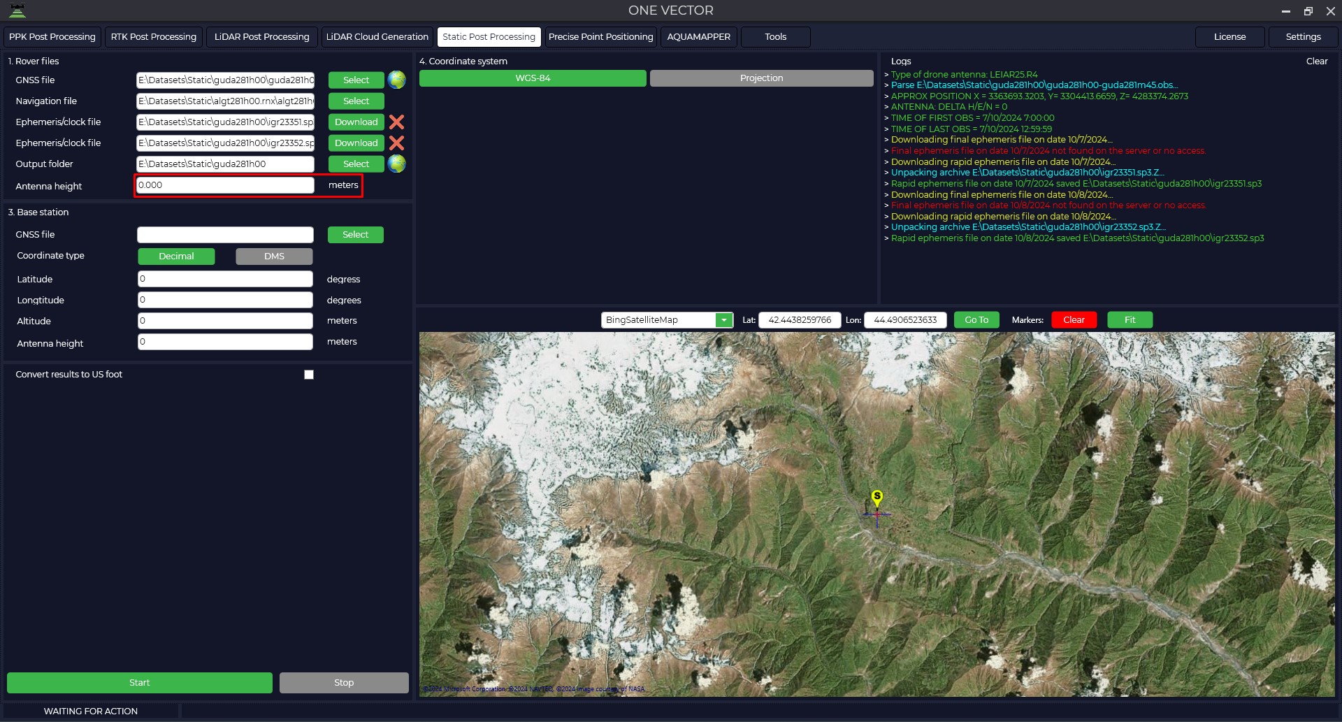
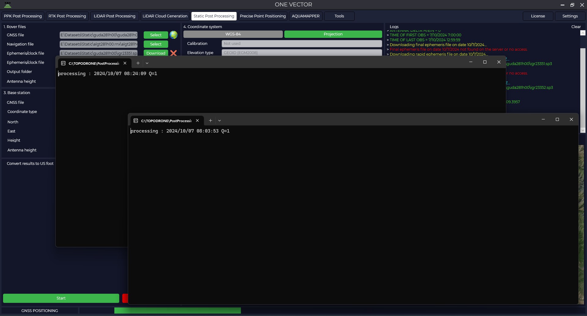
- To start this module it is necessary to open the TOPODRONE Post Processing program, go to the Static Post Processing tab and click on the "One vector" button.

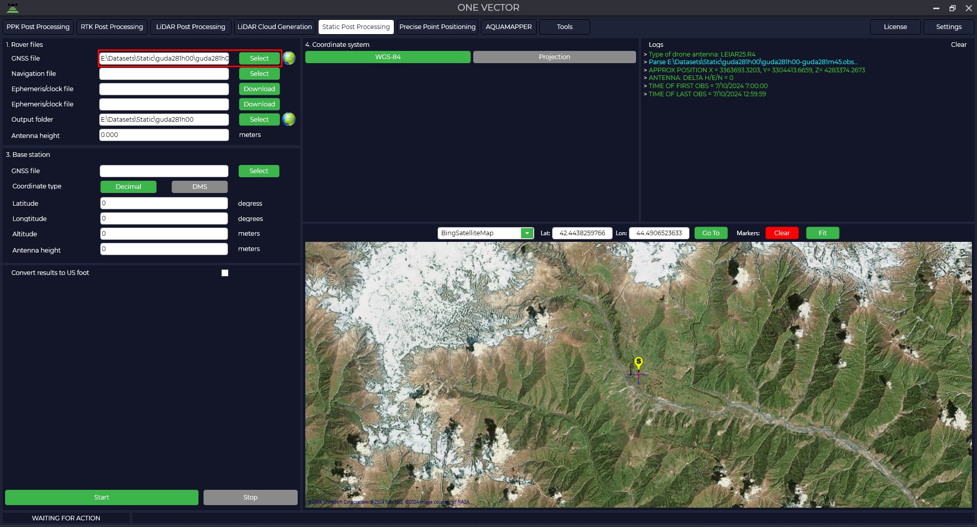
- Load measurement data from the rover.

- Download airborne ephemeris data.

- If necessary, download files of accurate ephemeris.

- Enter the height of the rover antenna.
The height of the antenna includes the height of the milestone or tripod from the measuring point to the bottom of the receiver mount and the height from the bottom of the receiver mount to the phase center.

- Download measurement data from the base station.

- After the files are uploaded, pressing the button allows you to analyze the quality of the data. For more information about data quality analysis, see Appendix B.
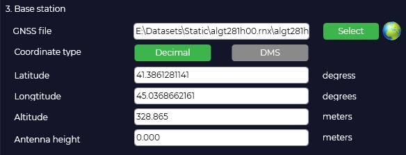
- The program will automatically load the coordinates and height of the base antenna from the Rinex file, taking into account that it was entered during measurement and display the location on the map.

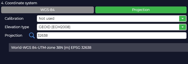
- In case your coordinate system is different from WGS-84, you need to click "Projection" button and select your coordinate system from the list or enter the coordinate system name in the search line, if necessary, select the geoid model. If your coordinate system is not in the list, you can add it to TOPODRONE Post Processing program.

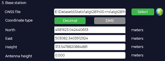
- Selecting a coordinate system will convert from WGS-84 to the projection of your choice. If necessary, correct the coordinates of the base station.
The height of the antenna includes the height of the milestone or tripod from the point of known coordinates to the bottom of the receiver mount and the height from the bottom of the receiver mount to the phase center.
After pressing the "Start" button, the program will proceed to calculations.

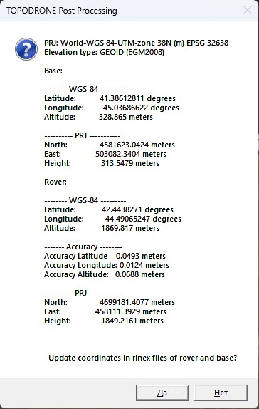
- Upon completion of calculations the program will display a window with coordinates of base station and rover in WGS-84 coordinate system and local coordinate system and will offer to save these data to observation files for further use of these data. Also in the output data folder the file with the calculation results will be saved.
Caption 
PRJ: World-WGS 84-UTM-zone 38N (m) EPSG 32638
Elevation type: GEOID (EGM2008)Base:
-------- WGS-84 ---------
Latitude: 41.38612811 degrees
Longitude: 45.03686622 degrees
Altitude: 328.865 meters
---------- PRJ -----------
North: 4581623.0424 meters
East: 503082.3404 meters
Height: 313.5479 metersRover:
-------- WGS-84 ---------
Latitude: 42.4438271 degrees
Longitude: 44.49065247 degrees
Altitude: 1869.817 meters
------- Accuracy --------
Accuracy Latitude 0.0493 meters
Accuracy Longitude: 0.0124 meters
Accuracy Altitude: 0.0688 meters
---------- PRJ -----------
North: 4699181.4077 meters
East: 458111.3929 meters
Height: 1849.2161 meters

Grid equalization
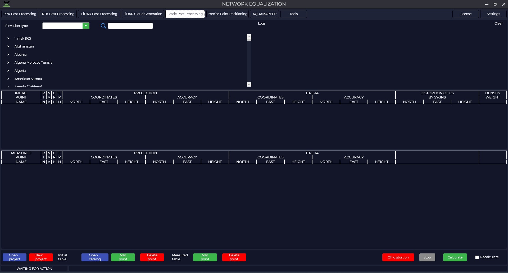
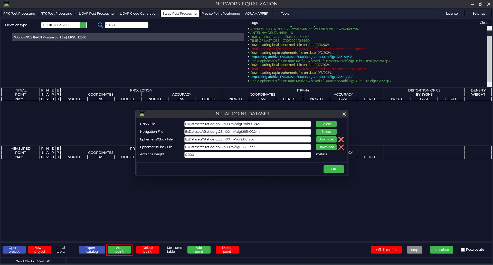
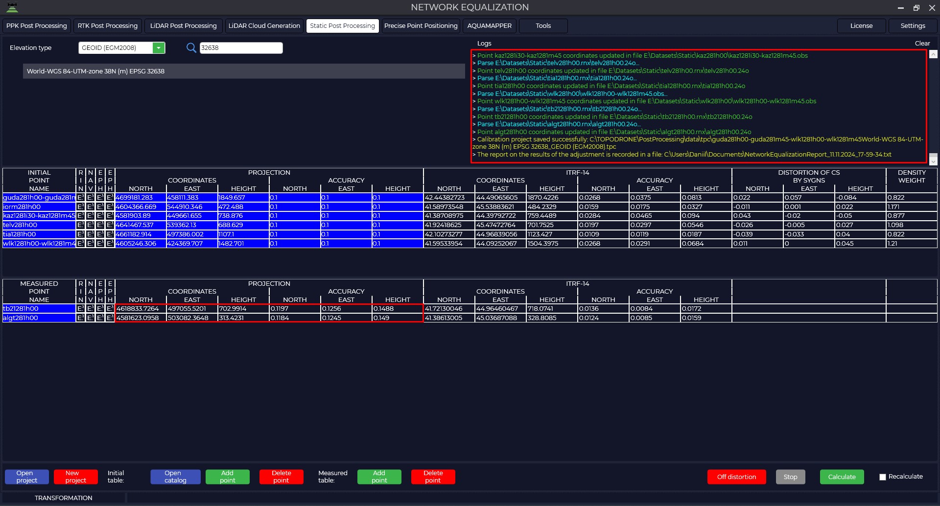
- To start this module, go to the Static Post Processing tab and click on the Network Equalization button.

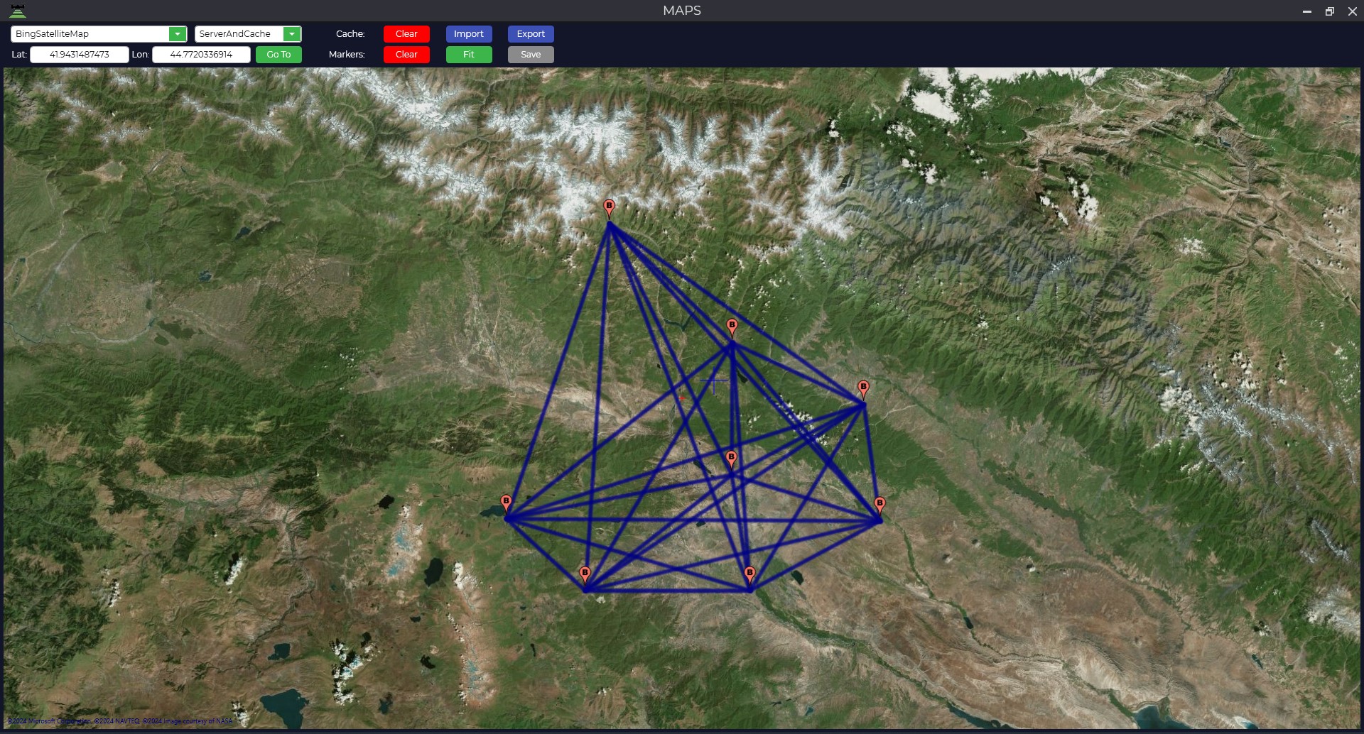
- To display the points where observations were made, the map window must be open at the time of file upload.

- The bottom panel has a number of tools: open or create a new project, open the source point catalog, add or delete source point files, add or delete measured point files, remove projection distortions, stop processing, and calculate.

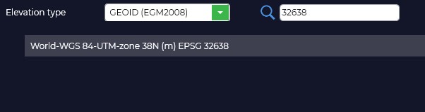
- The first thing to do is to select the required projection and the type of elevation to be used.

- When we click on the "Add Point" button next to the "Start Table" item, we need to load the data for the starting points.

GNSS file - a GNSS receiver measurement file in *.obs, *.rnx or *.*o formats.
Navigation file - navigation file of measurements in *.nav, *.rnx, *.n, *.p, *.g, *.h, *.q, *.c and *.l format.
Ephemeris file - file of final ephemeris in *.sp3, *.eph format, you can also upload a file of accurate flight clock *.clk. When you click on the Download button, if the data are available on the NASA server, the program will automatically download these data.
When processing the Grid Equation, the program uses the method of obtaining Precise Point Positioning (PPP) coordinates of the terrain using global navigation satellite systems by obtaining corrections to the orbital ephemeris and on-board clocks of all visible spacecraft. For the best calculation it is recommended to add daily measurements from the nearest reference base station or IGS.
Antenna height is the height from the center of the point to the phase center of the GNSS receiver.
Type Accuracy of orbits and clocks Accessibility Note Broadcast ~100 см
~5 ns RMS
~2.5 ns σIn real time GLONASS (.YYg) and GPS (.YYn) on-board ephemeris for a day in RINEX format summarized in the TsUP UltraRapid ~3 см
~150 ns RMS
~50 ns σIn 3-9 hours Refined ephemeris and corrections of airborne clocks Rapid ~2.5 см
~75 ns RMS
~25 ns σAfter 17-41 hours Ephemeris and corrections of onboard clocks obtained on the interval of last days Final ~2.5 см
~75 ns RMS
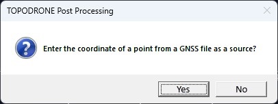
~20 ns σAfter 12-18 days Final ephemeris and flight clock corrections - When adding initial data to the program, a window will appear on entering coordinates of the point from the loaded file, click the "Yes" button.

- Then, if necessary, load the coordinate catalog of the source points or enter the coordinates and their accuracy manually.

If you do not know with what accuracy they have been determined, you should provide the following recommended accuracies:
• FAGS 20 mm north/east, 30 mm high;
• HCV 30mm north/east, 40mm high;
• AGS and GHS 40mm north/east, 50mm high;
• GGS 60mm north/east, 110mm high.
- To load the data for measured points, you must use "Add point" against the item "Measurement table" and perform the loading by analogy with the original points.

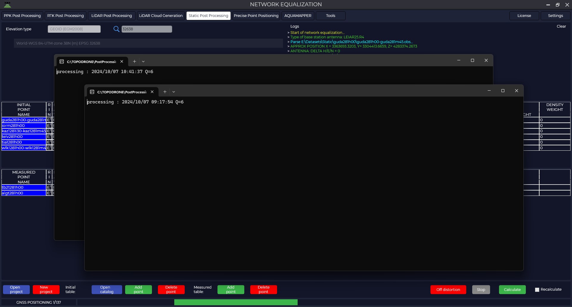
- Once all items have been loaded, click on the "Start" button and the program will begin the calculation. The number of operations and the total number of calculations to be performed will be displayed on the bottom left.
The calculation of the network follows the following algorithm:
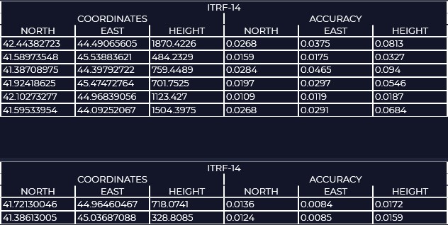
1) Calculation of coordinates of all points in ITRF2014 coordinate system by Precise Point Positioning - PPP method. After this step in the ITRF-14 window you will see the calculated coordinates and their accuracy.
2) In the next step, the program performs Precise Point Positioning and static measurement of all possible vectors, performs point coordinates calculation by precision weighting.
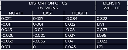
3) Then, using the coordinate system and coordinates of the initial points, taking into account the weighting accuracies of the points, the program calculates the total displacement from the parameters of the selected projection and creates a grid of residual distortion corrections. - In the DISTORTION OF CS BY SYGNS window you can see the residual distortions of the coordinate system relative to the original points. In the DENSITY WEIGHT window Density of points, it is needed to increase/decrease the weight of distortions, a single point has a higher weight than a point that is next to others.

-
As a result of calculations you will get a catalog of coordinates of points in the coordinate system that was specified, accuracy of determination of these coordinates and distortion grid for use in the TOPODRONE Post Processing program. The calibration file can be opened through the "Tools" module, "Calibration" tab. In addition, a report of the processing results will be saved in the document folder.

- When you click the "Correct Distortion" button, the program distributes the errors to the source items and re-runs the processing.

- The table below summarizes the results of processing
Caption Until distortion is eliminated After removing distortion 








Precise Point Positioning
Precise Point Positioning (PPP) — is a global navigation satellite system positioning method that calculates coordinates with an error of only a few centimeters under good conditions. PPP is a combination of several relatively sophisticated GNSS positioning refinement methods. Unlike the RTK method, which uses a base station, a rover and relatively small distances between them, the PPP method uses a single GNSS receiver.
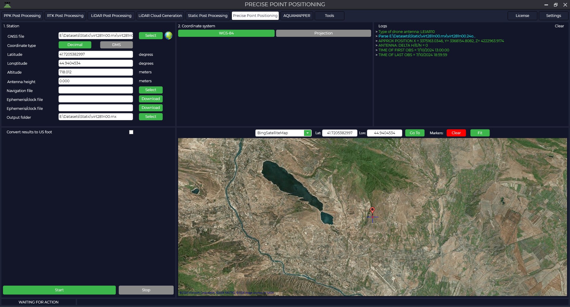
- Click on the Precise Point Positiong tab to use this module and click on the "Select" button to download data from the GNSS receiver. Supported formats: *.ubx, *.obs, *.rnx and *.*o.

- Next we need to upload the rest of the data.

Navigation file - navigation file of measurements in *.nav, *.rnx, *.n, *.p, *.g, *.h, *.q, *.c and *.l format. Ephemeris/clock file - final ephemeris file in *.sp3, *.eph format, it is also possible to upload exact on-board clock file *.clk. When you click on the Download button, if the data are available on the NASA server, the program will automatically download these data.
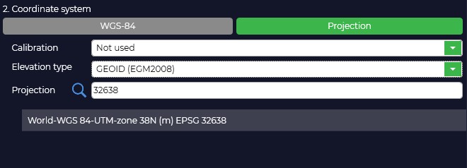
Output folder - folder with output data, it can be changed if necessary. - Select the coordinate and altitude system in which we need to get the coordinates of the point.

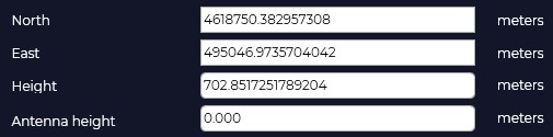
- Then, if data is available, enter the coordinates of the base station and the antenna height, taking into account the phase center.

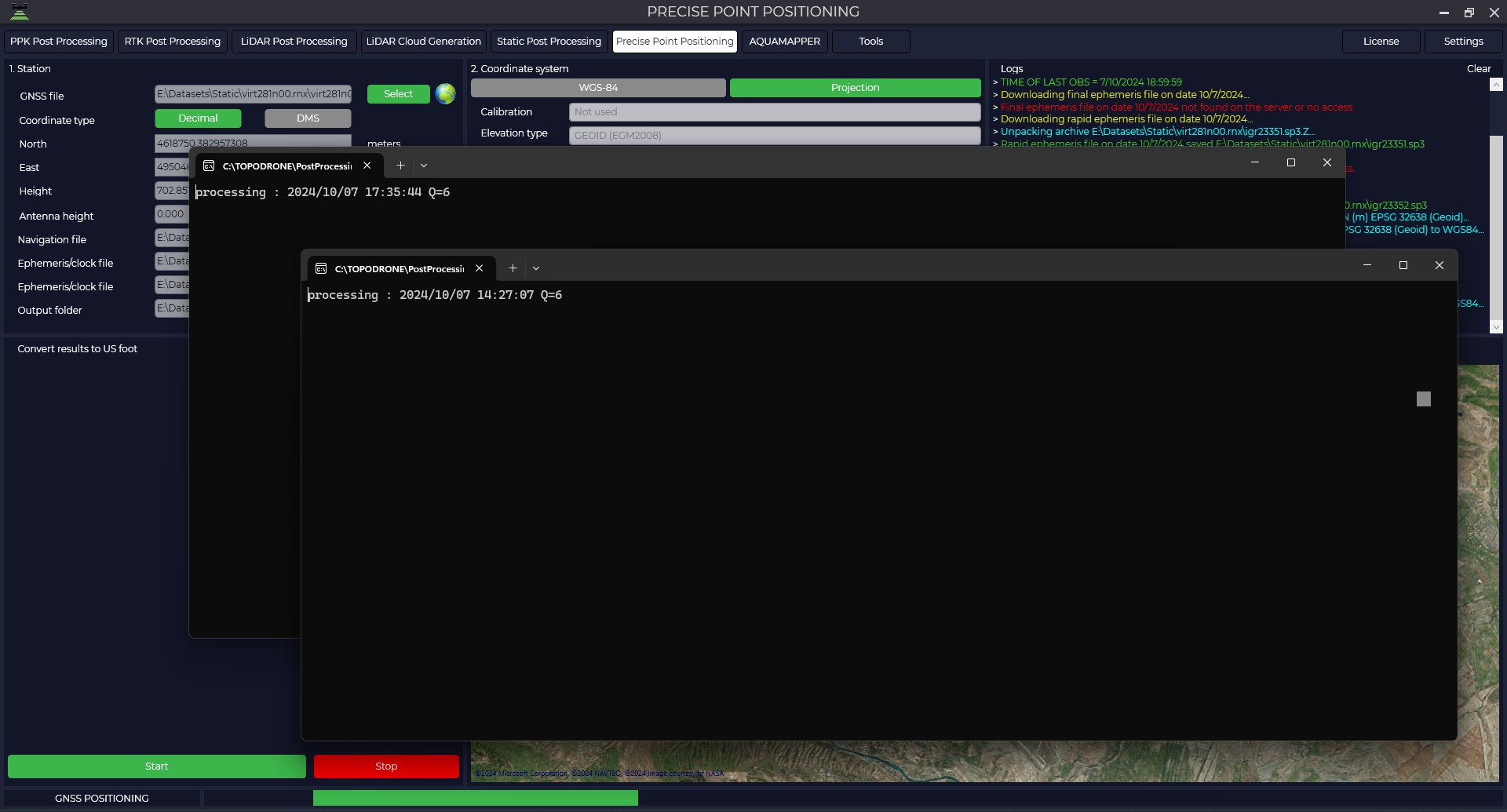
- When you click on the "Start" button, the program will start calculations.

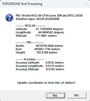
- As a result of calculations, a window will appear with the coordinates of the point in the WGS-84 coordinate system, in the selected coordinate system and the accuracy of these coordinates. Also, if you click on the "Yes" button, the program will write the calculated coordinates in the header of the rinex file.

AQUAMAPPER
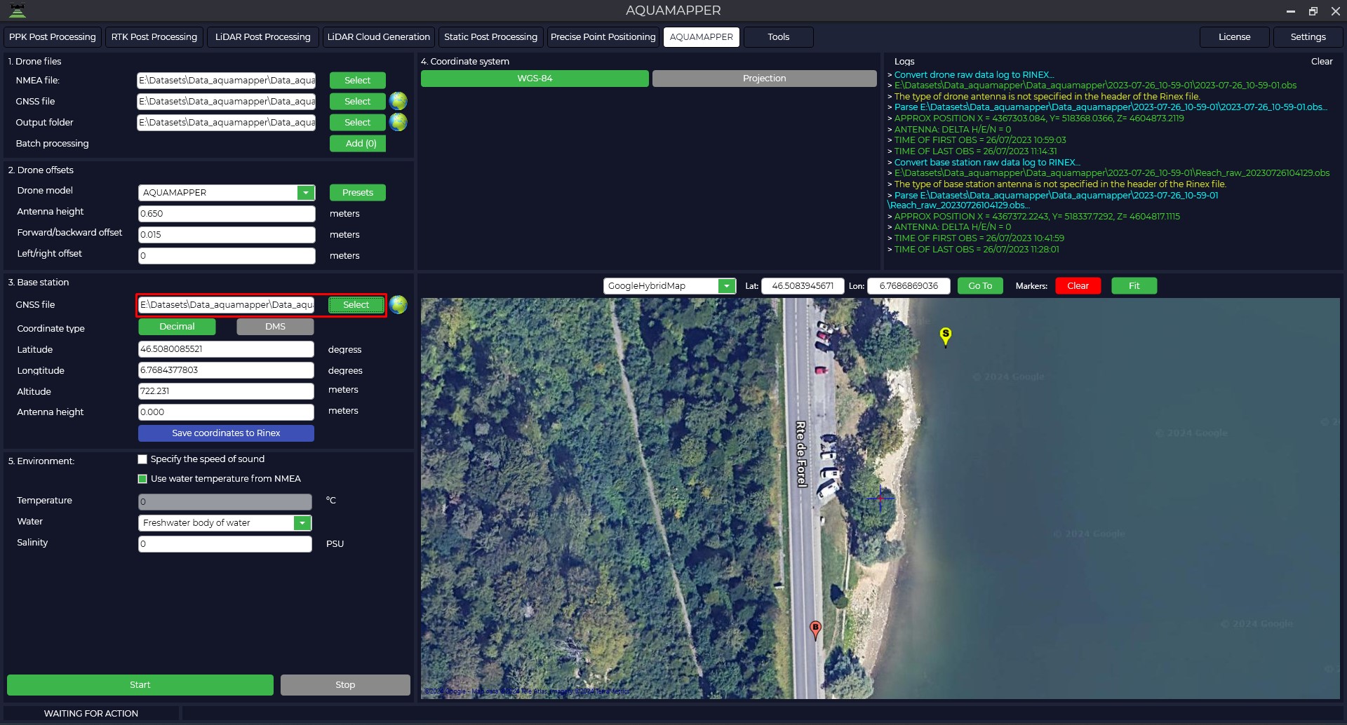
This module is designed for processing data obtained using the TOPODRONE AQUAMAPPER bathymetric scanner. To process the data, follow these steps::
- Launch the TOPODRONE Post Processing program and go to the AQUAMAPPER tab.

- Select the .nmea file that you received from the bathymetric scanner during data collection. The file from the GNSS receiver will load automatically, and a path to the folder with the processing results will be created.

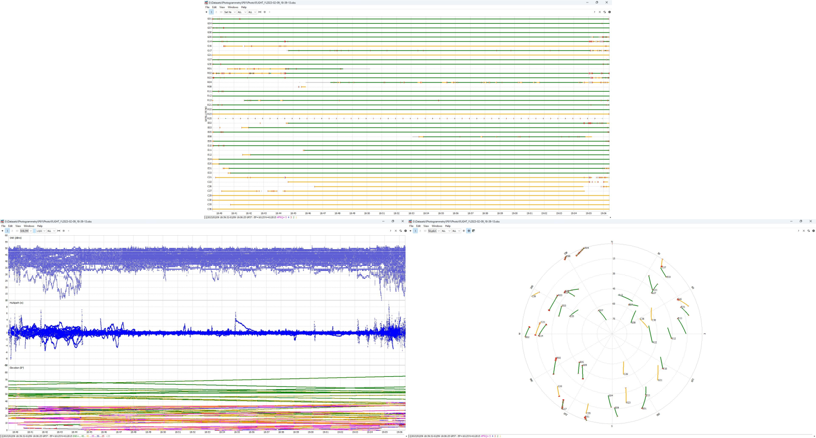
- By clicking on the button , you can analyze the data quality. For more information about data quality analysis, see Appendix B.
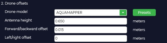
- On the "Drone offsets" tab, if necessary, specify the antenna offset relative to the bathymetric sensor. If necessary, you can add your own data by clicking on the "Presets" button and entering the desired offsets.

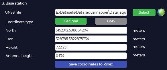
- Select the file from the base station (*. ubx, *obs, *rnx, *YYo). For files in the *rnx and *ubx formats, the conversion process to *obs format will automatically start. The program automatically loads the coordinates of the base station and the height of the base antenna from the Rinex file, if they were specified during the measurement.

The Logs window displays information about the program's actions. Pay attention to the recording time of files from the rover and base station. The base station file must be older than the rover files.
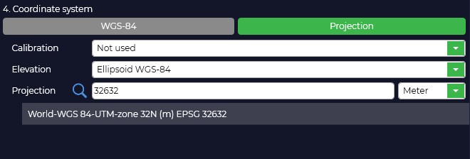
- Select a rectangular coordinate system. To do this, click the "Projection" button and select a coordinate system from the list or enter its name in the search bar.
If the desired coordinate system is not in the list, you can add it to the TOPODRONE Post Processing program. When you select a coordinate system, the conversion from WGS-84 to the selected projection occurs. If necessary, adjust the coordinates of the base station.

- Change the type of height used. When you select the type, the height will be automatically converted.
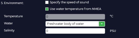
- Specify the environment type. There are two options: specify the speed of sound for correct calculation, or specify the salinity of the reservoir and its temperature. The temperature can be taken from the bathymetric sensor by checking the box "Use water temperature from NMEA".

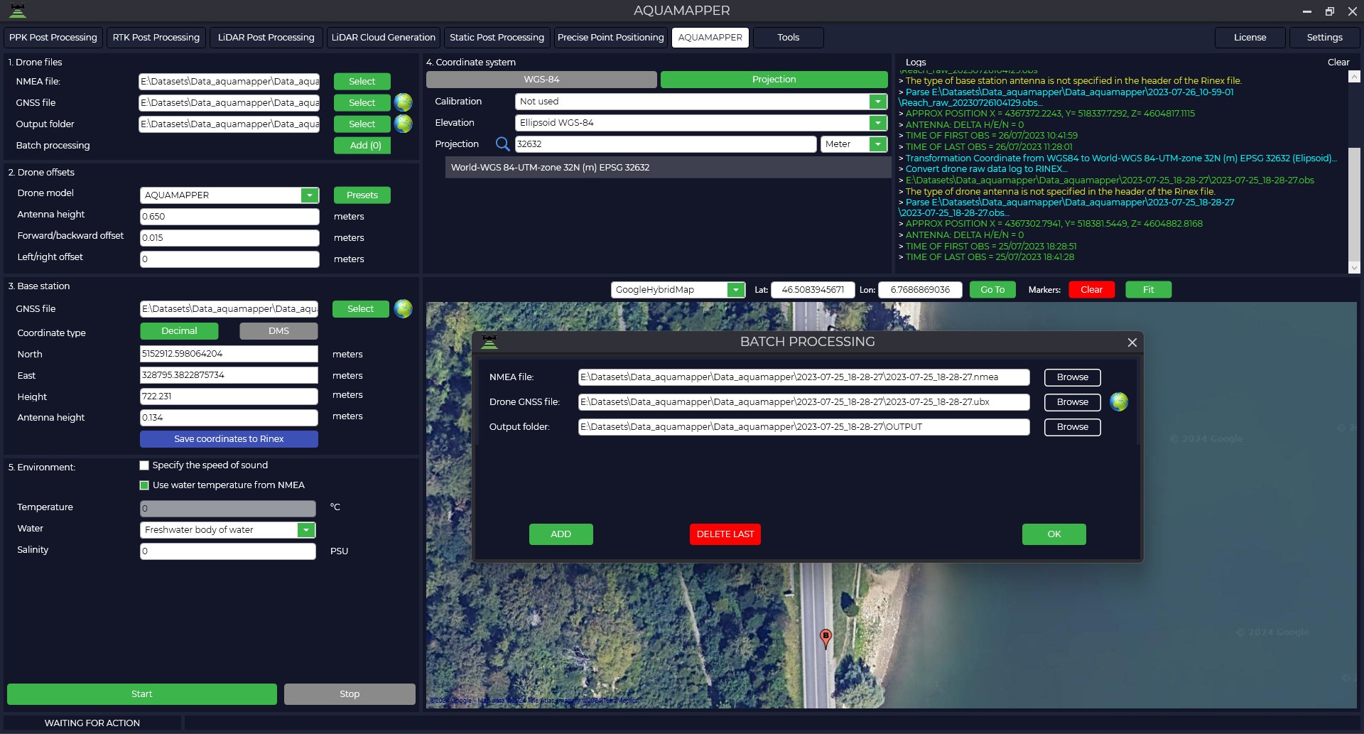
- The TOPODRONE Post Processing program allows you to process multiple data sets from a single base station within a single observation session. For batch processing, click "Add (0)" and add additional files .nmea and click "OK".

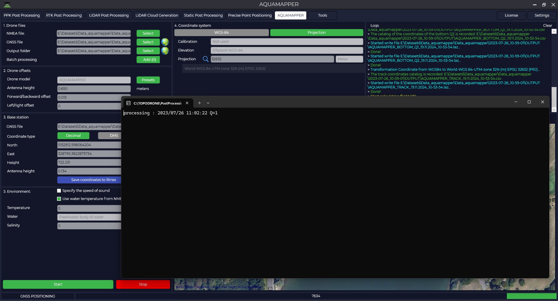
- To start processing, click the "Start" button. Data processing takes place simultaneously in the forward and reverse directions, and the solution type is displayed as the letter " Q " with a number: Q1 — fixed solution, Q2-floating solution, Q5-no solution.

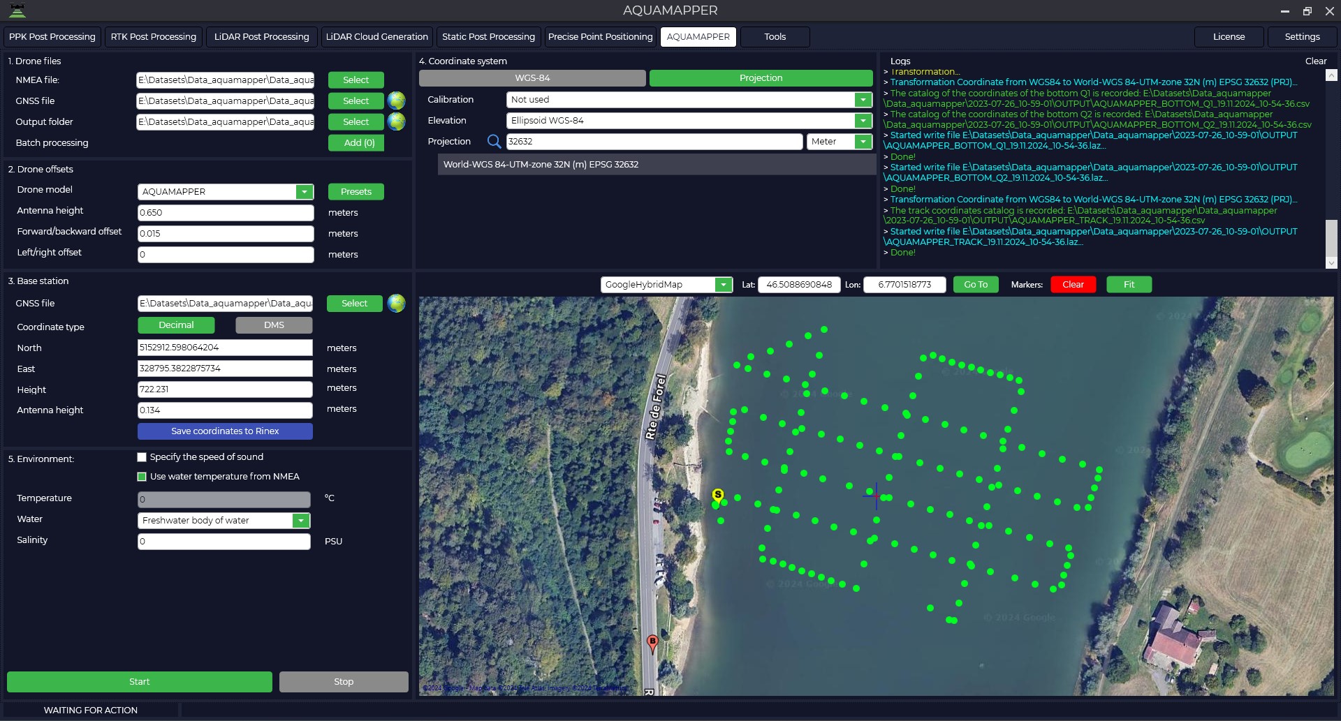
- As a result of processing, the AQUAMAPPER trajectory will be displayed on the screen and a set of files will be generated.

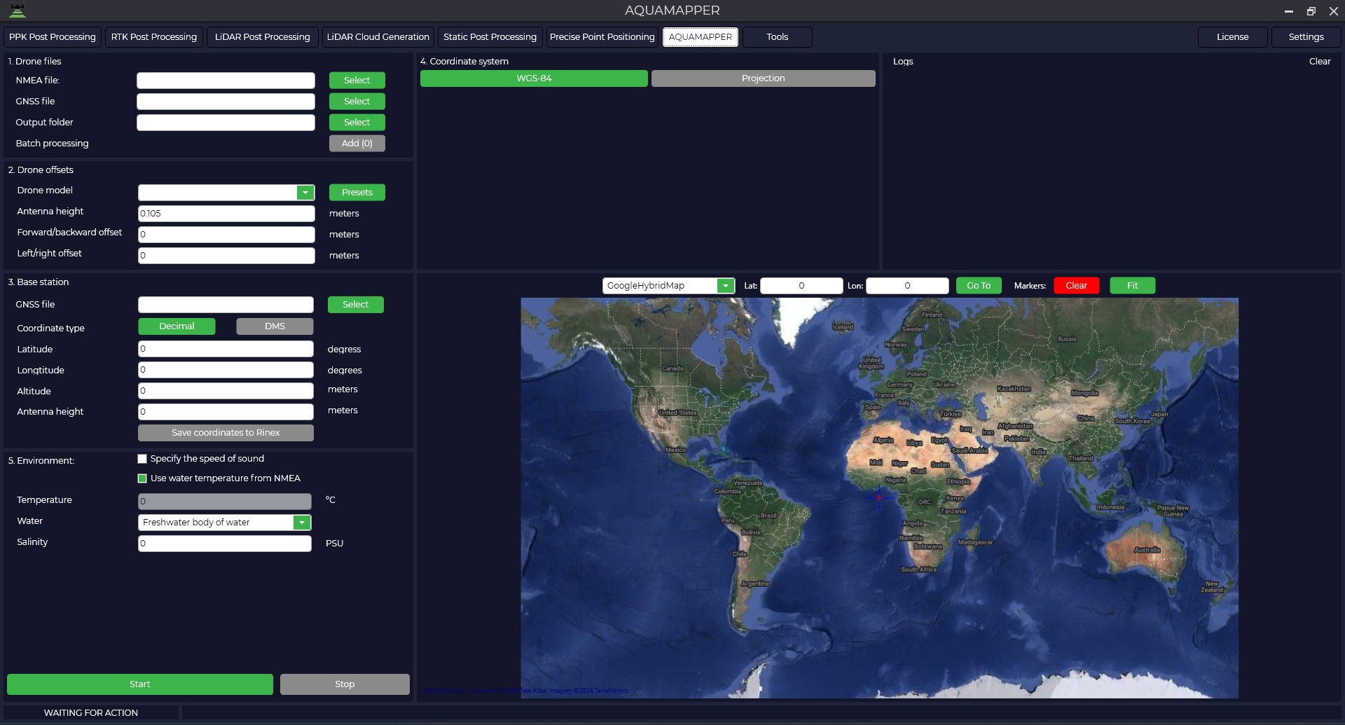
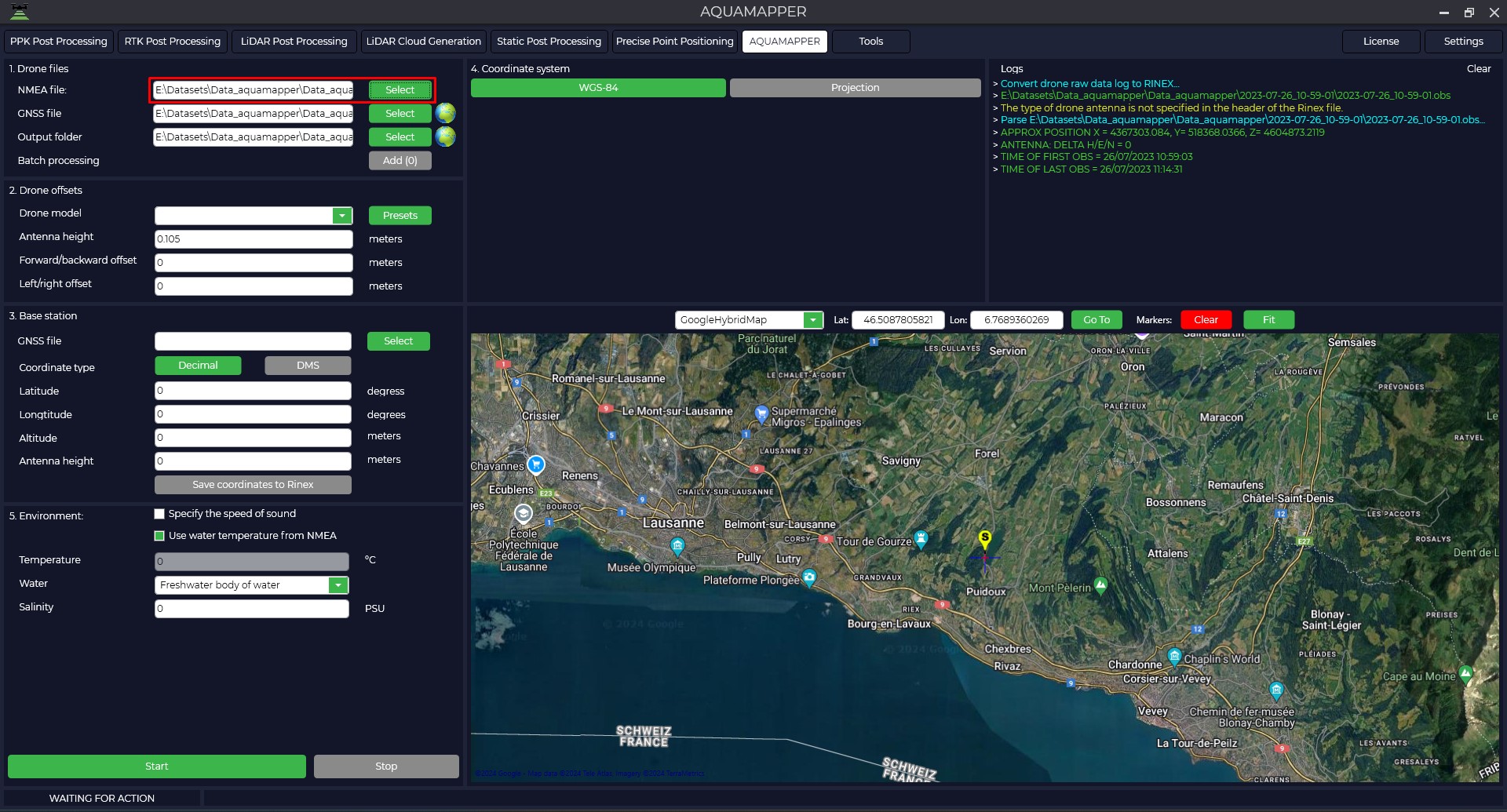
|
|
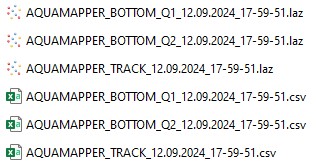
Data is written in two formats:*. laz and *. csv. Files with the TRACK prefix contain information about the trajectory, and files with the BOTTOM prefix contain information about the topography of the reservoir bottom. |
Two graphs will also be displayed: the upper graph shows the slope of the bathymetric sensor at a certain point in time, and the lower graph shows the depth. 
Then, based on the data obtained, you can build a depth map.

Tools
This part of the instructions will cover the various tools that help make the job easier.
Filters LAS/LAZ
When launching the filters, we are greeted with a startup window.
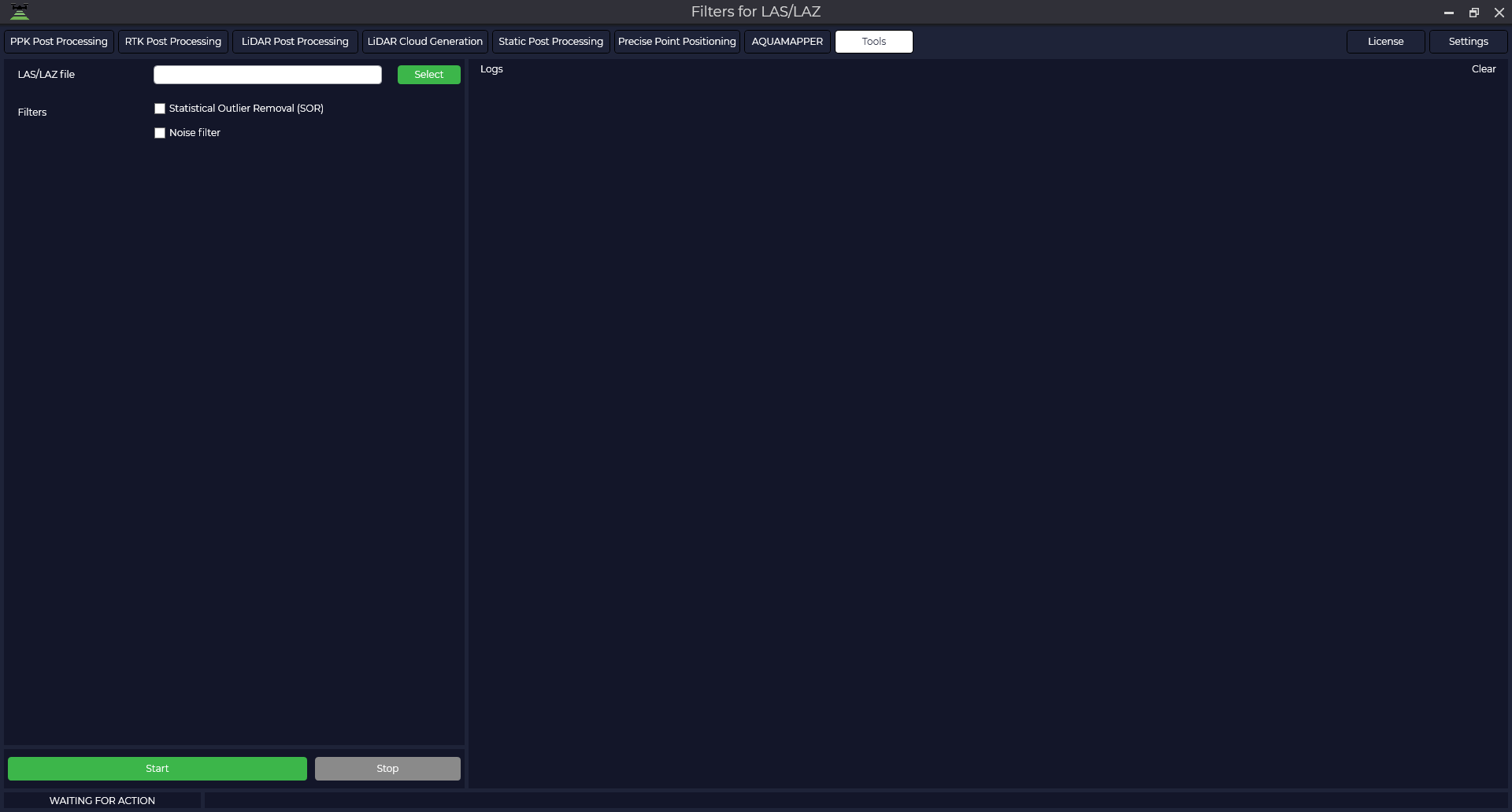
Statistical Outlier Removal (SOR) is a method that first calculates the average distance between each point and its neighbors. It then removes points that are more than the average distance plus a few standard deviations. The minimum number of neighboring points is 6 and the standard deviation is 1.
Noise removal is a method that is similar to statistical outlier removal (SOR), but it considers the distance to the main surface rather than neighboring points. It locally fits a plane around each cloud point and removes a point if it is too far from that plane. This filter can be thought of as a low-point filter.
Surface reconstruction is a technique that is used to create complete surface models from heterogeneous data. Sometimes small errors in distance measurements can lead to difficulties in removing anomalies by statistical analysis. In such cases, surface reconstruction uses a resampling algorithm that attempts to reconstruct missing parts of the surface by polynomial interpolation between surrounding data points. This corrects small errors and smooths out artifacts such as "double walls" that occur when multiple scans are recorded simultaneously.
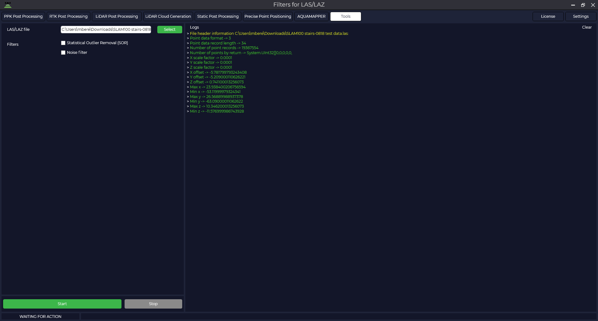
If you select a file in LAS or LAZ format, the login window will display the information contained in the file: number of points, X, Y, Z offsets, etc.
To process, check the required filters and press the "Start" button. If several filters are selected, they are applied sequentially. All results are saved to the folder with the source file.
Ground classification
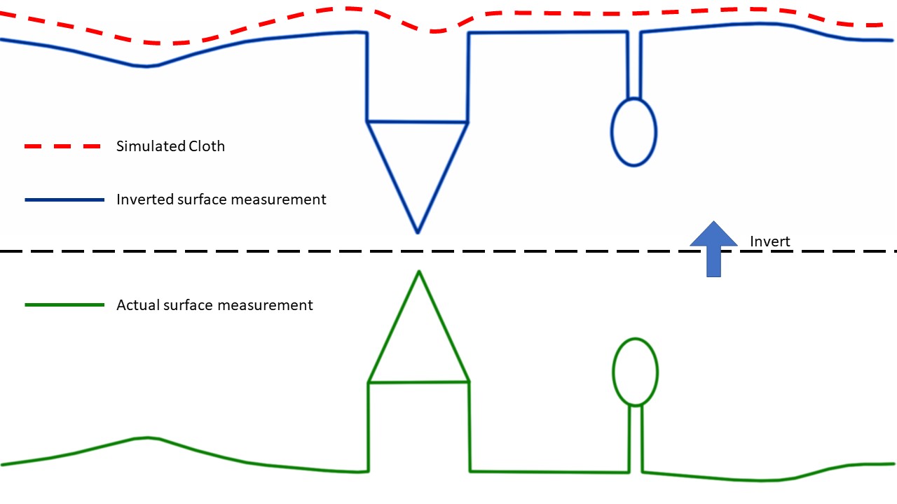
The Ground Classification tool allows you to divide the point cloud into two components: terrain related points and all other points. This method is based on a simplified physical process. Imagine a piece of cloth suspended above the terrain, which then falls down due to gravity. If the fabric is soft enough, it will stick to the surface and the final shape of the fabric will be a digital model of the terrain. However, if the point cloud is first turned upside down and the fabric is made stiff, the final shape will be a digital terrain model. A method called fabric modelling is used to model this process. Based on this method, a cloth modelling filtering (CSF) algorithm has been developed to extract ground points from the point cloud. An overview of the proposed algorithm is shown in Fig. First, the original point cloud is flipped upside down, and then a fabric is dropped on the flipped surface. By analysing the interaction between the fabric nodes and the corresponding points, the final shape of the fabric can be determined and used to classify the original points into terrain points and all other points.
When launching the tool, we are greeted with a startup window.
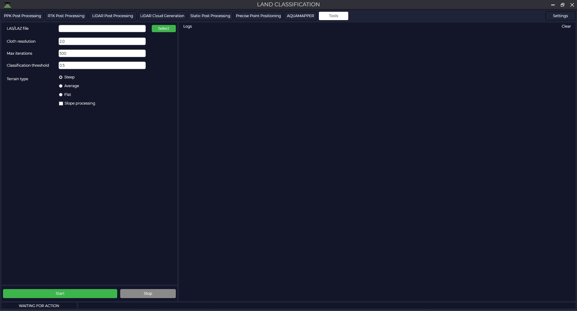
In the window that opens, click the "Select" button and select the file in the *.las or *.laz format for which you are going to make a classification. The Logs window displays information about the uploaded file.
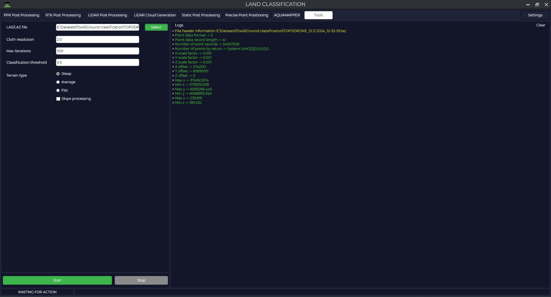
After that, set parameters that match the characteristics of your point cloud:
The grid step is the size of the grid cell, expressed in point cloud units, that is applied to cover the terrain. Increasing the grid resolution will result in a more detailed surface model, but will increase the computational load.
Number of iterations - the maximum allowable number of iterations performed during surface modelling. For most scenes it is recommended to set this value at 500 iterations, which is sufficient to achieve acceptable accuracy.
Classification tolerance - a parameter used to separate point clouds into ground related points and other points based on distances to the modelled terrain surface. The units of the tolerance must match the units of your point cloud. The recommended value for this parameter is 0.5, which is appropriate for most processing scenarios.
Terrain Type - with this parameter you can set the type of point cloud scene.
For steep slopes, this algorithm can produce relatively large errors because the modelled fabric is above the steep slopes and does not agree well with ground-based measurements due to internal constraints between particles.
Slope handling — the problem described above can be solved by selecting this option. If your scenes don't have steep slopes, just ignore it.
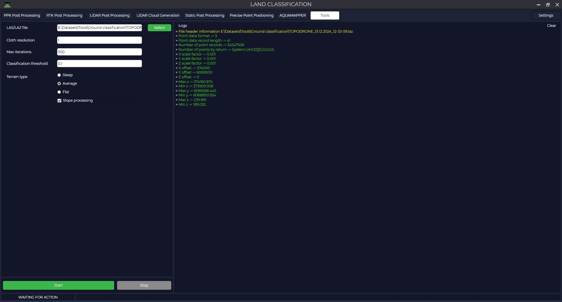
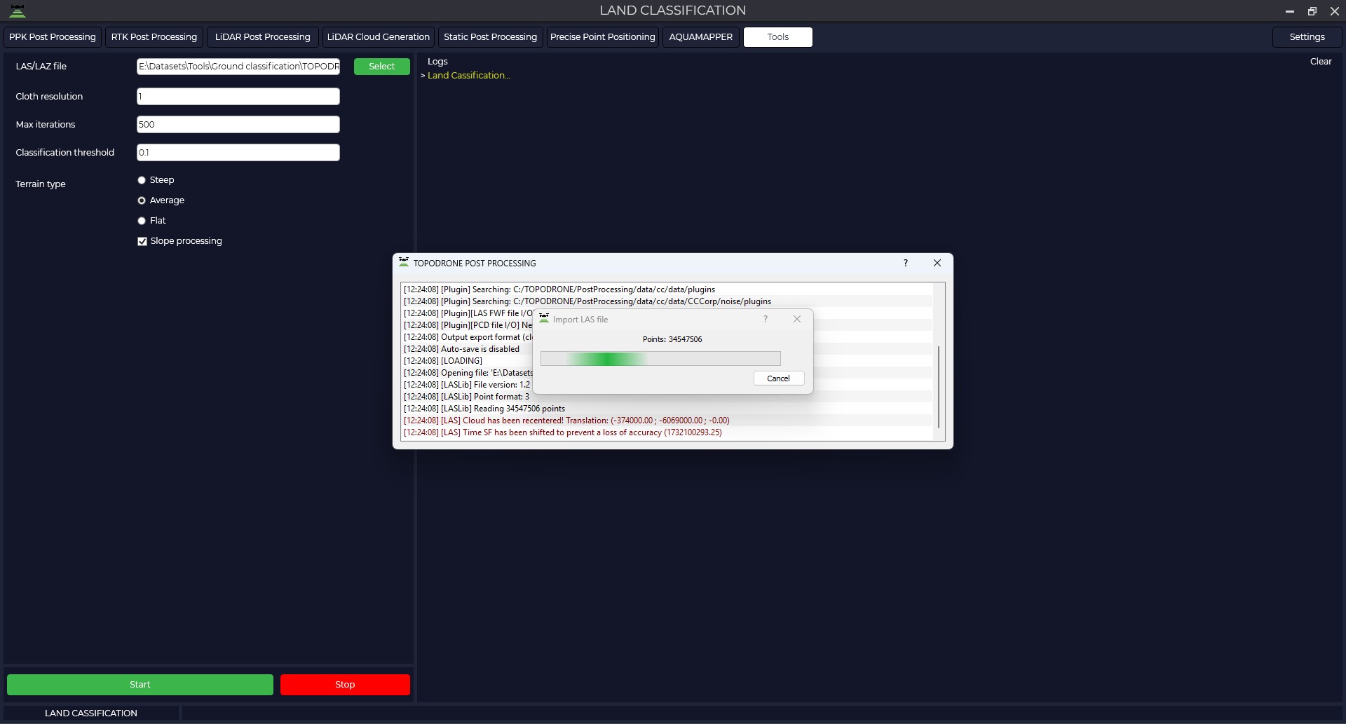
Press the ‘Start’ button and wait for the operation to complete.
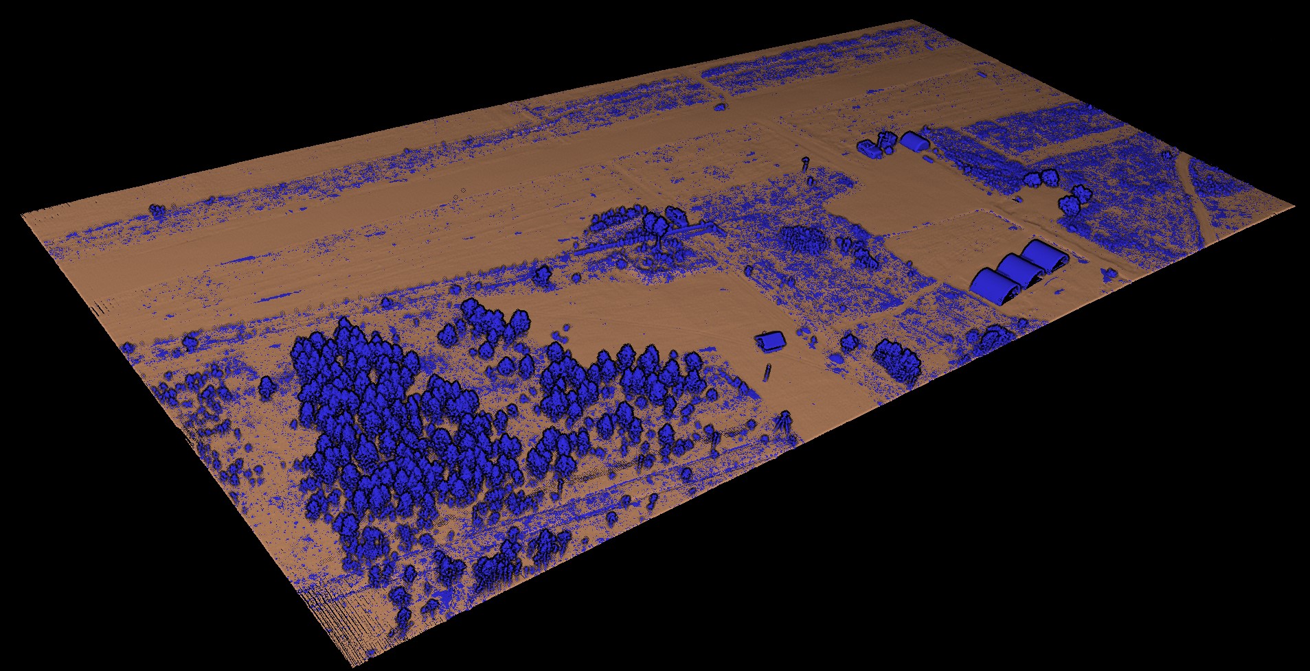
The final result is the files: the ground point cloud and the rest of the points.
LAS/LAZ Insta 360 Coloring
This module is designed for automatically assigning color characteristics to a Mobile Laser Scanning (MLS) point cloud, coloring it with natural colors using data obtained from TOPODRONE scanning systems.
Operating Principle and Data Requirements:
To obtain a point cloud with reliable RGB information, the following processing sequence must be executed:
-
Primary Data Processing: Perform standard processing of raw data in the LiDAR Post Processing module to obtain the laser scanner's trajectory.
-
Point Cloud Generation: Generate the final point cloud in LAS/LAZ format using the LiDAR Cloud Generation module.
-
Point Cloud Coloring: At the final stage, using the "LAS/LAZ Insta 360 Coloring" tool, RGB values are assigned to the points in the cloud. The algorithm matches each laser reflection point with the corresponding pixel from the panoramic images taken by the Insta 360 camera, based on the precise trajectory and data about the camera's position relative to the laser scanner. This ensures realistic coloring in natural colors.
The point cloud coloring process involves several stages.
Data Preparation
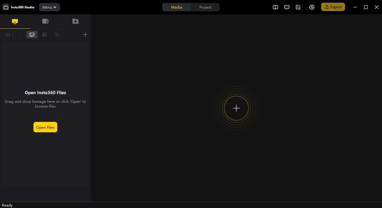
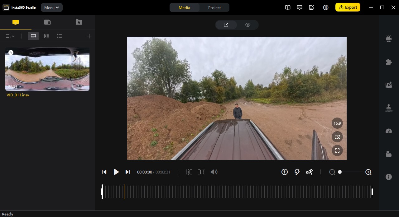
During recording, the Insta 360 camera saves data in its proprietary formats (*.lrv and *.insv). These formats are optimized for working with panoramic video in the manufacturer's software. For further processing, specifically for point cloud coloring, the video stream must be converted to the standard *.mp4 format. To do this, you need to install the Insta360 Studio program.
-
Launch the Insta360 Studio program.

-
Import the source files (*.lrv and *.insv) into the project.

-
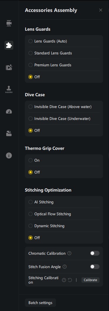
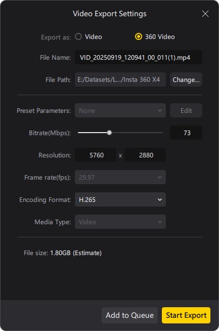
Navigate to the "Accessory Layout" tab and set the parameters according to the screenshot below.

-
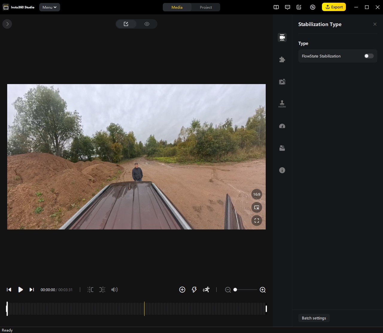
In the "Stabilization Type" tab, deactivate the "FlowState Stabilization" option by unchecking the corresponding box.

-
Initiate the export of the video file using the settings specified below into the folder containing the source *.lrv and *.insv files.

Point Cloud Coloring Process
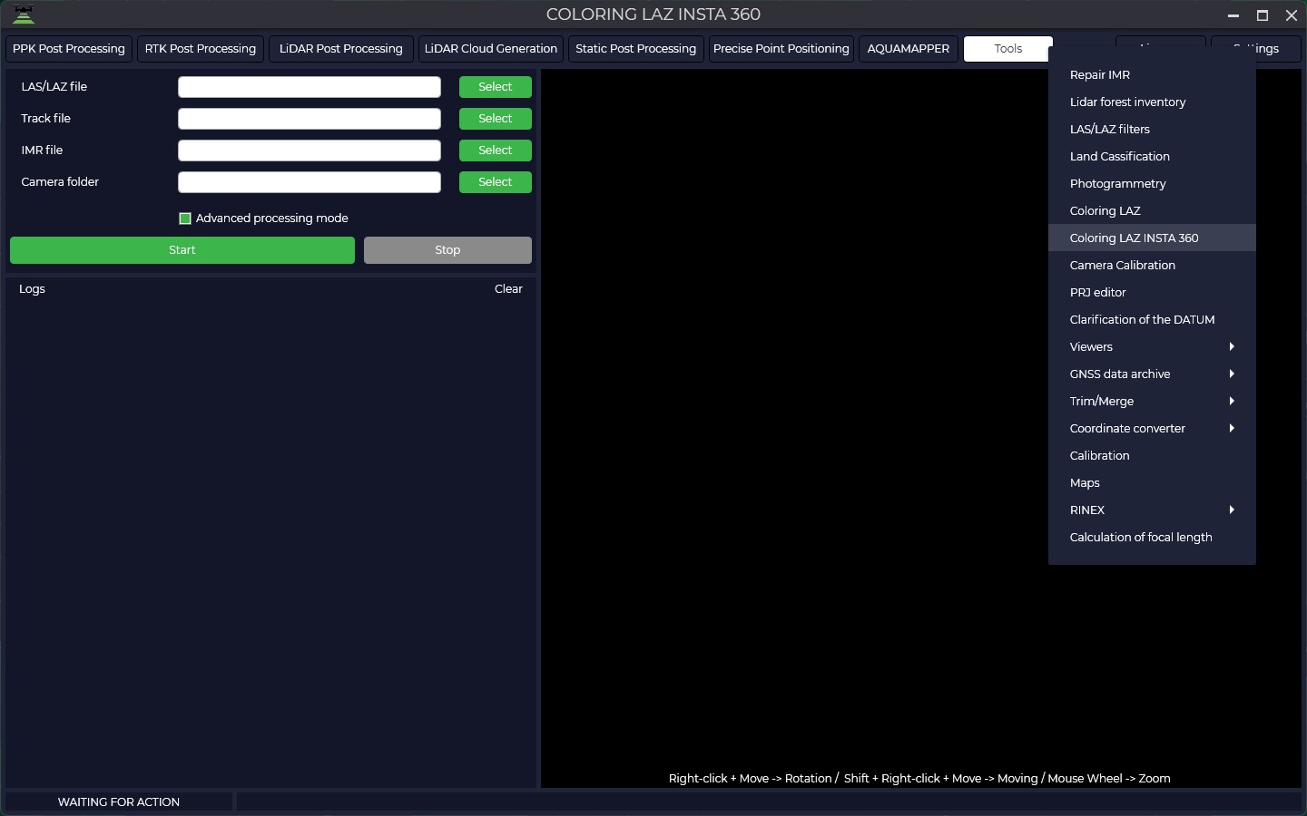
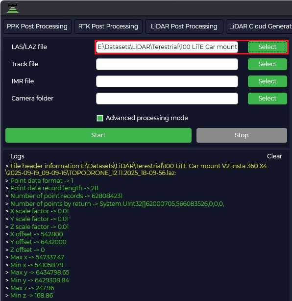
Specify the point cloud file in LAS/LAZ format, generated in the previous processing step in the "LiDAR Cloud Generation" module. This is an uncolored point cloud that contains spatial coordinates (X, Y, Z) and other laser information but lacks color attributes.
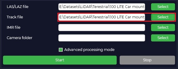
Select the trajectory file in the appropriate projection, obtained along with the point cloud from the "LiDAR Cloud Generation" module. The trajectory file contains precise coordinates and orientation of the scanning system at each moment in time. This data is critical for the temporal and spatial synchronization of frames with the cloud points.
Load the Inertial Measurement Unit (IMU) data file.
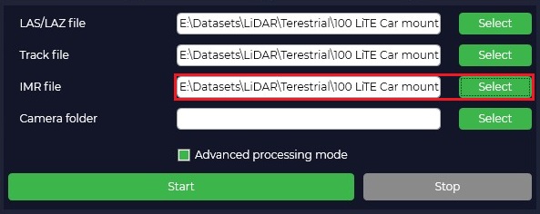
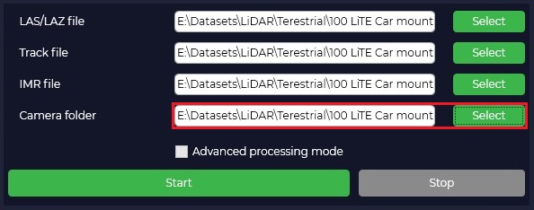
Specify the folder containing all the necessary video materials in *.lrv, *.insv, and *.mp4 formats.
Click the "Start" button to initiate the coloring algorithm.
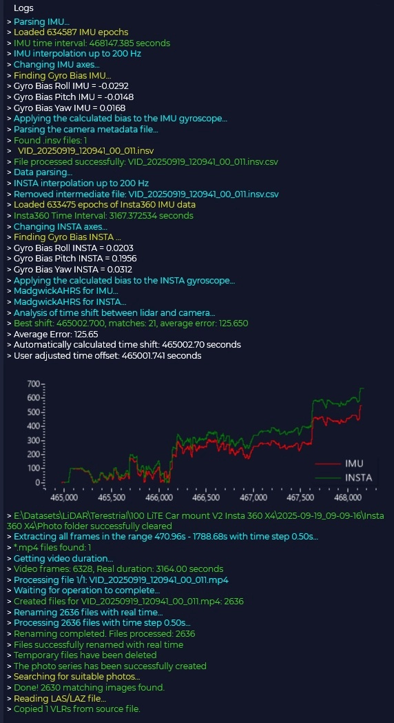
The processing progress is displayed in the "Log" text window. This window outputs information messages, warnings, and errors.
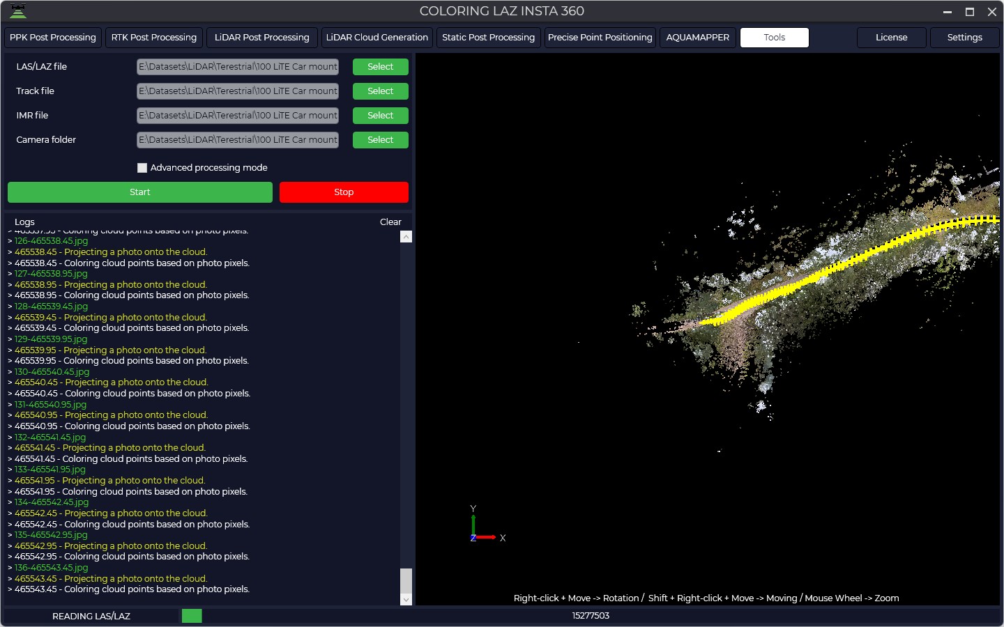
The "Viewer" window displays the process of assigning colors to the point cloud points in real-time, allowing for visual control over the processing accuracy.
Upon successful completion of the process, the module will automatically create a new file of the colored point cloud. The file is saved in the same directory as the source cloud. The prefix _RGB is added to the source filename for identification. A folder named "Photo" will be created in the directory containing the video files; this folder will contain panoramic images georeferenced to the WGS-84 coordinate system.
PRJ editor
PRJ Editor is a tool that allows you to edit the coordinate system knowing the transition parameters. In order to use it you need to select "PRJ Editor" in the Tools panel.
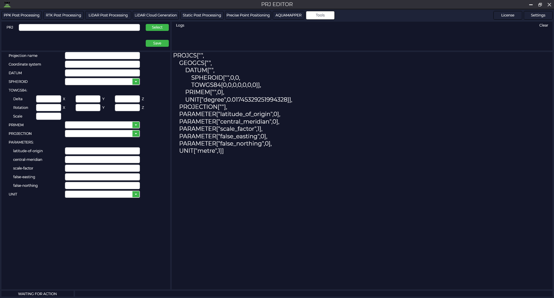
Currently, a small amount of photogrammetry and laser scanning software supports affine transformations, so this tool does not support affine transformations in the same way.
In the window that opens, click the "Select" button and select the *.prj file you want to edit.
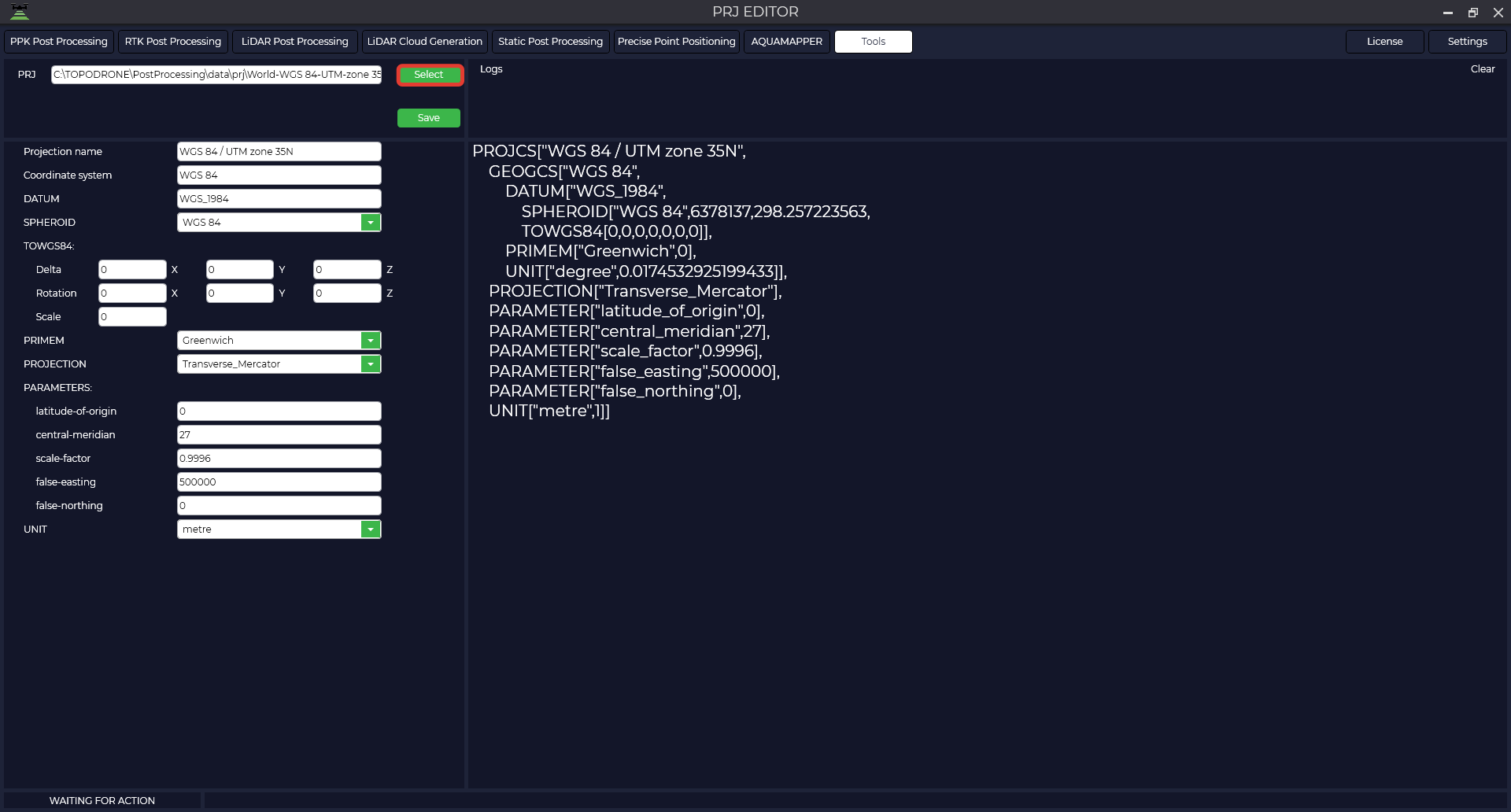
The table provides a description of the parameters
| Projection name |
WGS 84 / UTM zone 35N | Projection name |
| Coordinate system | WGS_1984 | Name of coordinate system |
| DATUM | WGS_1984 | Datum name |
| SPHEROID | WGS 84",6378137,298.257223563 | Name of ellipsoid |
| TOWGS84 | 7 parameters of transition to WGS84 | |
| Delta | 0,0,0 | Displacement of the intermediate geocentric coordinate along the X, Y, Z axes. It is specified in meters, and the translation direction is indicated by the value sign. |
| Rotation | 0,0,0 | The amount of rotation about the X, Y, Z axes that applies to intermediate geocentric coordinates. It is specified in angular seconds, and the direction of translation is indicated by the sign of the value. |
| Scale | 0 | A scaling factor that applies to intermediate geocentric coordinates. The value is given in parts per million and is the difference between the actual scaling factor and one. For example, a scale parameter value of -2.5 gives an actual scale factor of 0.9999985. That is, the actual scale factor used is obtained by multiplying the parameter value by 1.0x10-06 and adding the result (algebraically) to 1.0. |
| PRIMEM | "Greenwich",0 | Zero meridian, indicating the offset between the zero meridian of the declared coordinate system and the Greenwich coordinate system. |
| UNIT | "degree",0.01745329251994328 | The unit of measure of SC (degrees). |
| PROJECTION | Transverse_Mercator | Projection type |
| PARAMETERS | ||
| Latitude of origin | 0 | Initial latitude |
| Central meridian | 27 | Central meridian |
| Scale factory | 0.9996 | Scale factor |
| False easting | 500000 | Shift east |
| False northing | 0 | Shift north |
| UNIT |
metre |
Projection unit |
Make all necessary changes to the parameters, click the "Save" button, specify the path to save and the file name.
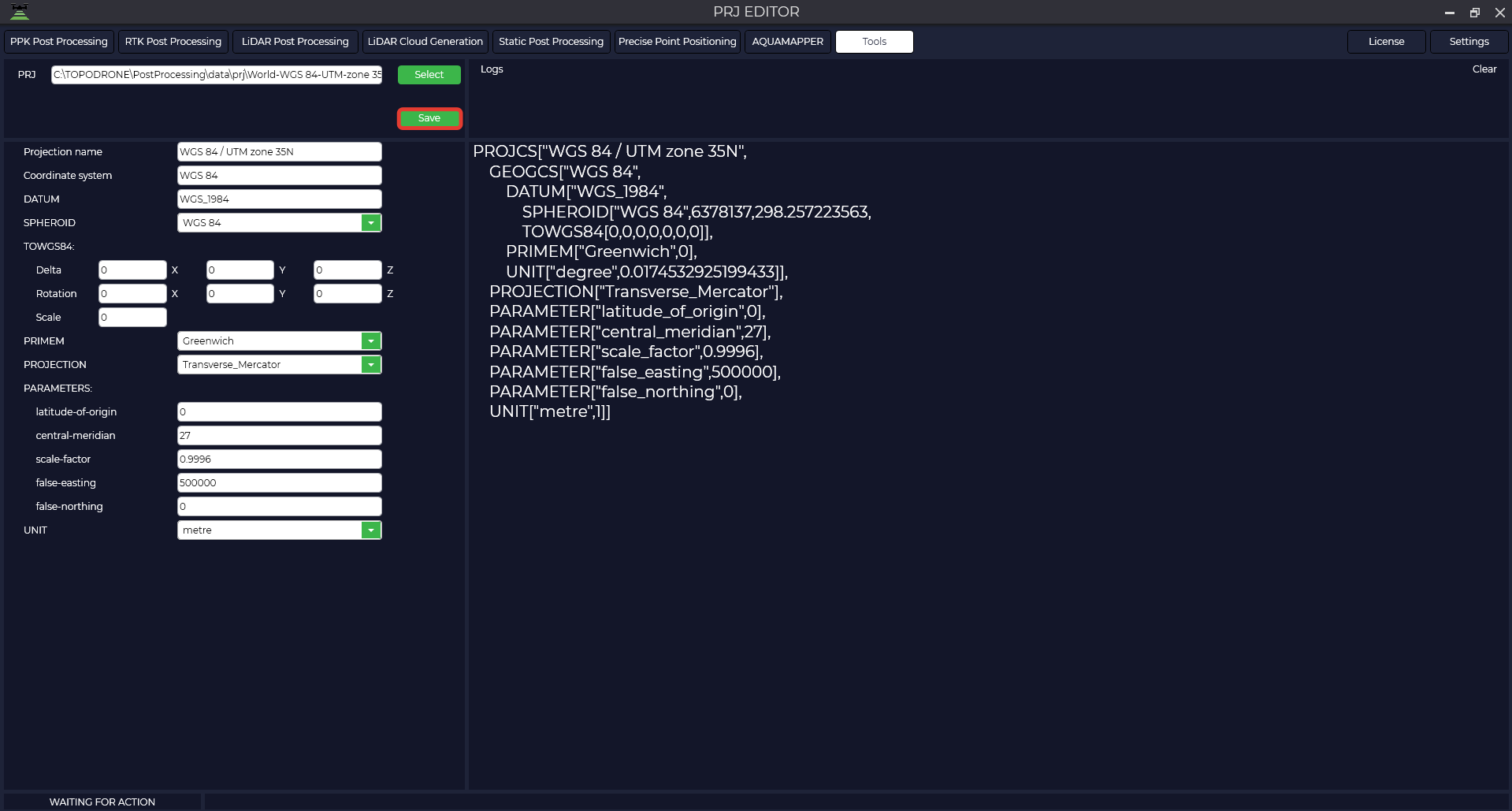
The resulting file is shown below.
PROJCS["WGS 84 / UTM zone 35N",
GEOGCS["WGS 84",
DATUM["WGS_1984",
SPHEROID["WGS 84",6378137,298.257223563,
TOWGS84[0,0,0,0,0,0,0]],
PRIMEM["Greenwich",0,
UNIT["degree",0.0174532925199433,
PROJECTION["Transverse_Mercator"],
PARAMETER["latitude_of_origin",0],
PARAMETER["central_meridian",27],
PARAMETER["scale_factor",0.9996],
PARAMETER["false_easting",500000],
PARAMETER["false_northing",0],
UNIT["metre",1]]Viewing the point cloud
This tool is intended for viewing and analyzing the point cloud obtained during processing in TOPODRONE Post Processing software. To start the module, go to the Tools tab, then Viewers and click on the New button. If you need to open a point cloud that has just been closed, select Previous. In the opened tab select the point cloud in *.las or *.laz format. After loading, the point cloud will be displayed in the main window.
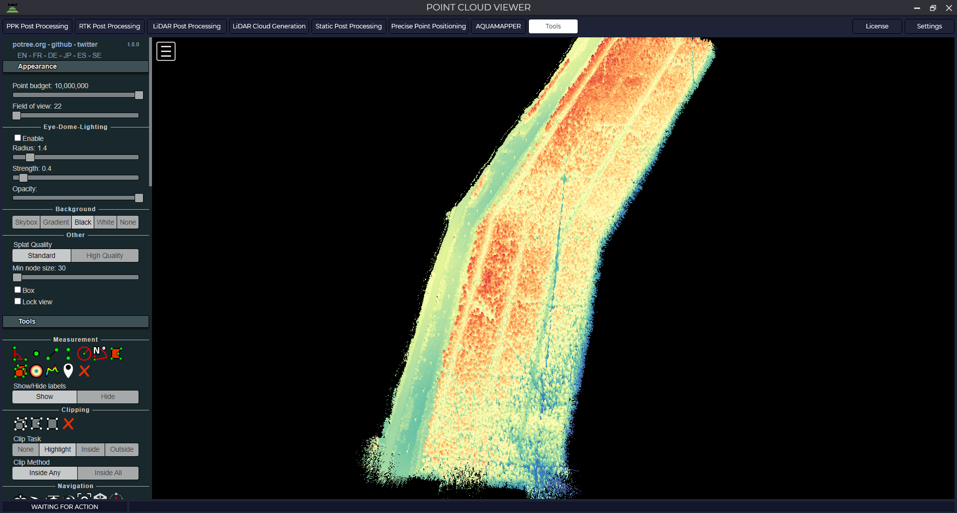
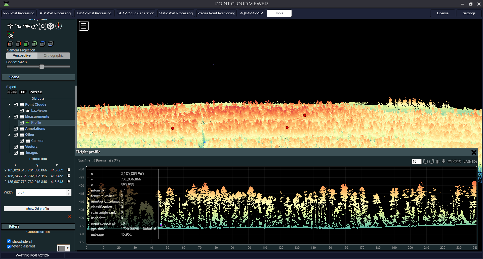
Data archive GNSS
This module is a large database with publicly available base stations for downloading observation files.
- To start the module, go to the "Tools" tab, then "GNSS Data Archives" and select the database you need.

- Then download the data from your receiver to have the program select the date and time of the base stations or enter this data manually. Specify the folder where you want to save the result.

- In the table or on the map, select the base station from which you want to download data and press the "Start" button, the data download will start in the folder you specified.

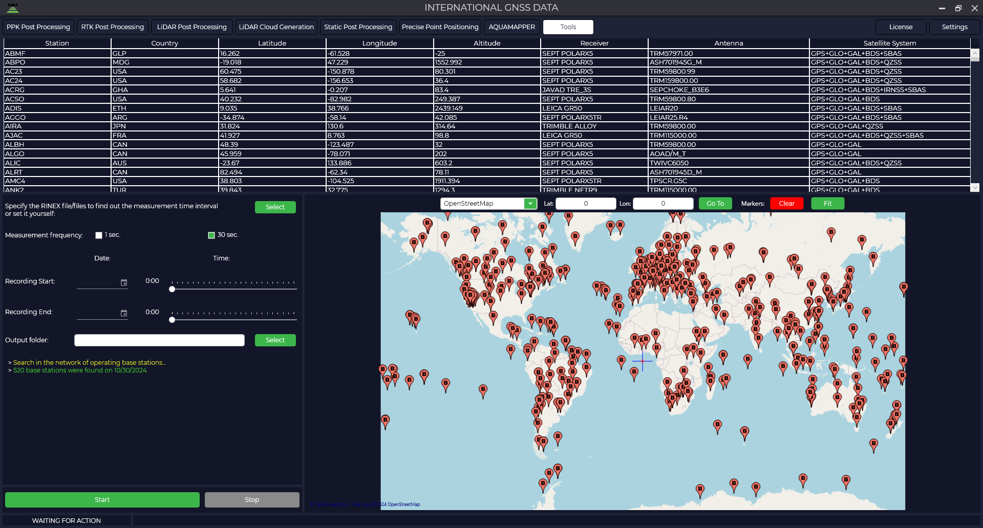
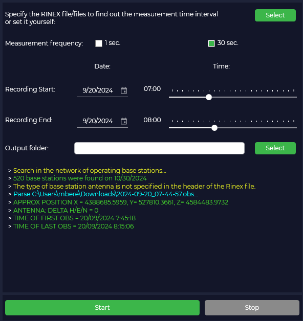
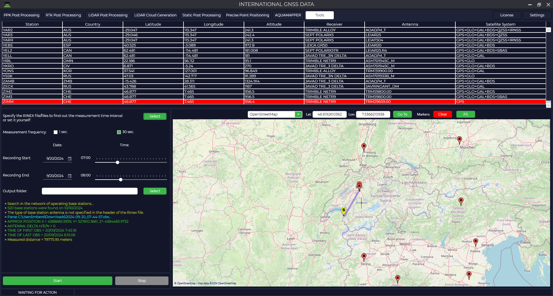
Track trimming
This tool is designed to trim a trajectory file in *.pos and *.poses format.
To start the tool, select Track Trim in the Tools, Trim/Stitch tab. Then select the track you want to trim.
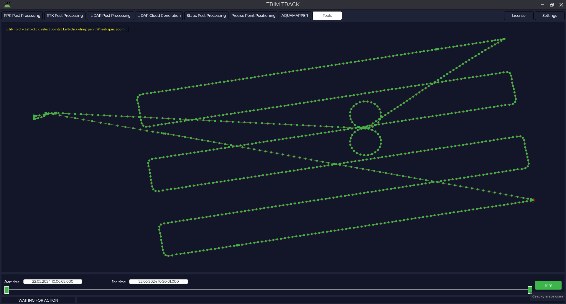
There are two sliders at the bottom, by moving them you specify the interval of the trajectory, which will remain and which will be cut. You will see a visual representation of the two colors on the trajectory. Green indicates the area that will be saved after trimming, and red indicates the area that will be trimmed.
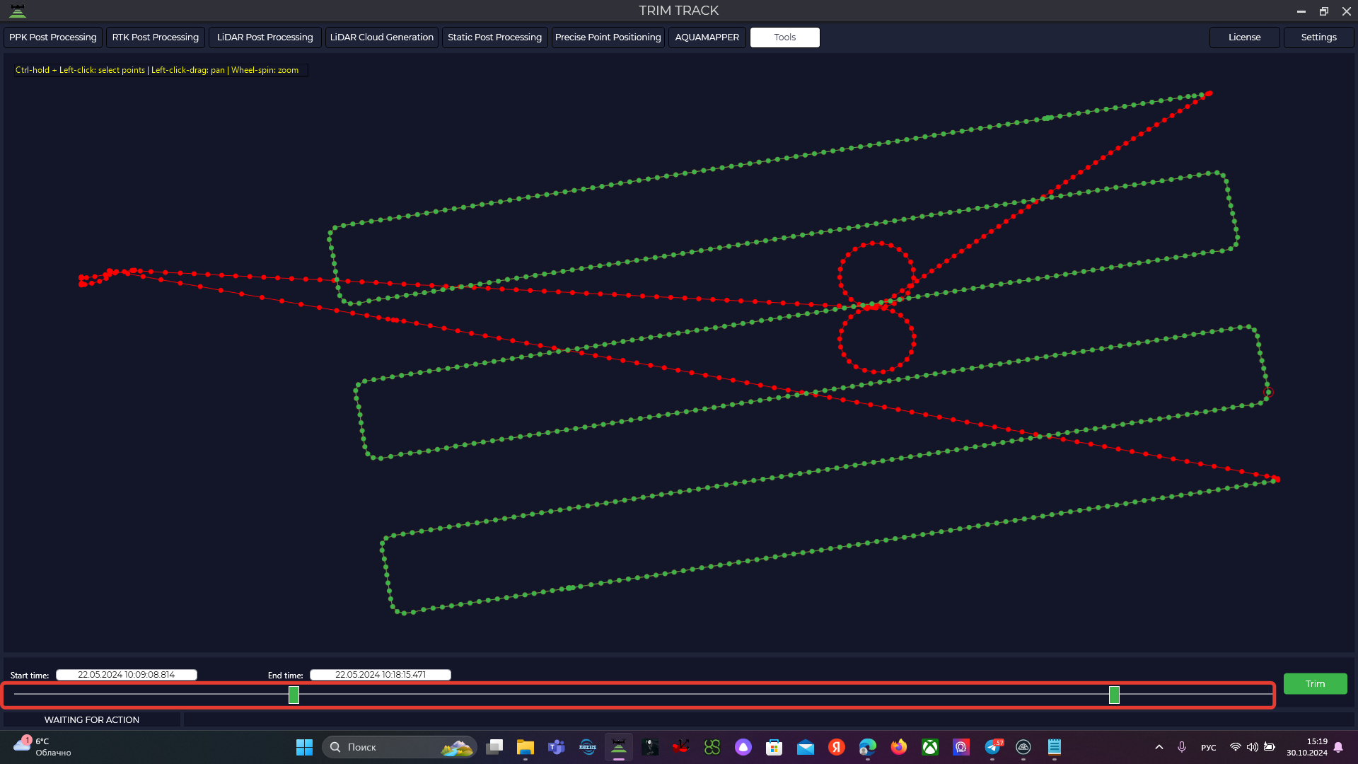
After selecting an area, cut the part you don't want by clicking on "Trim". The trajectory will be saved to a file in the original format.
Merge track files
The module is designed for trajectory stitching followed by point cloud generation in the LiDAR Cloud Generation module.
To start the tool, select Track File Stitching in the Tools, Trim/Stitch tab. Then through the "Add" button select the trajectories to be merged.
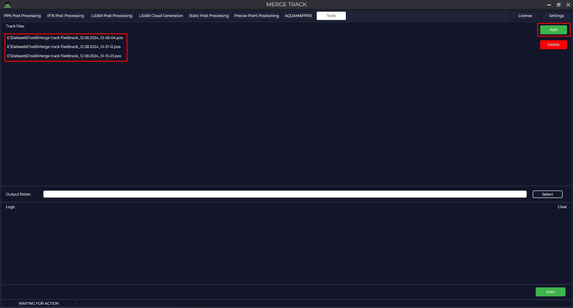
Select the Output folder where to save the merged trajectory and click "Start" to start the process. At the end of the process the program will display a message that everything is ready.
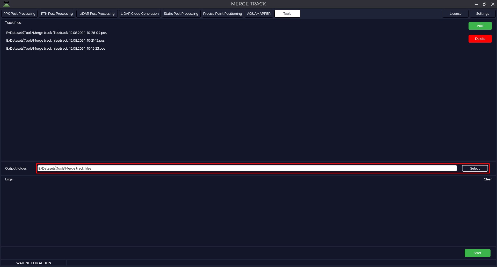
Trim IMR (+GNSS)
You can use the IMR(+GNSS) Trim IMR(+GNSS) tool to eliminate jumps in inertial navigation system (IMU) data when working in conjunction with satellite navigation data.
This tool is useful if after starting trajectory processing the dataset contains an error message - IMU file contains gaps in measurement points! Use the "Trim IMR(+GNSS)" tool to remove the missing sampling time interval.

To start the tool, select IMR(+GNSS) Trim in the Tools, Trim/Stitch tab. Then select the file in *.imr format to be trimmed and the GNSS receiver file.


The program will pre-process the GNSS and if there were any gaps in the IMU data, you will see this on the screen as vertical lines and the designation (Gap).
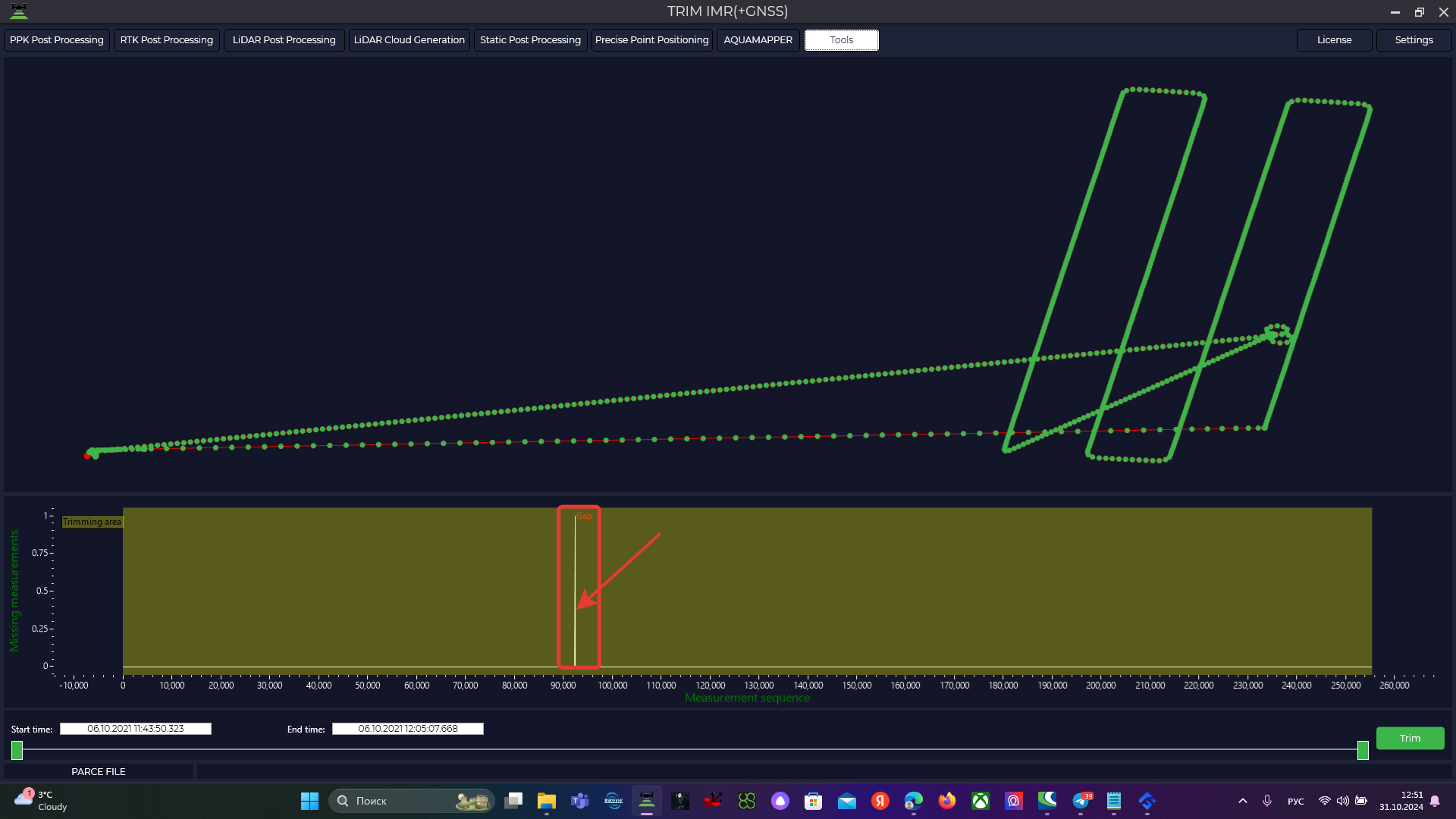
For further correct processing, it is required to exclude outliers from the data.
From the selected file we will need to exclude two skips from processing, therefore the IMU file should be divided into three segments and further processed in three parts. Only one segment is trimmed, so in this case we will need to repeat this procedure three times.
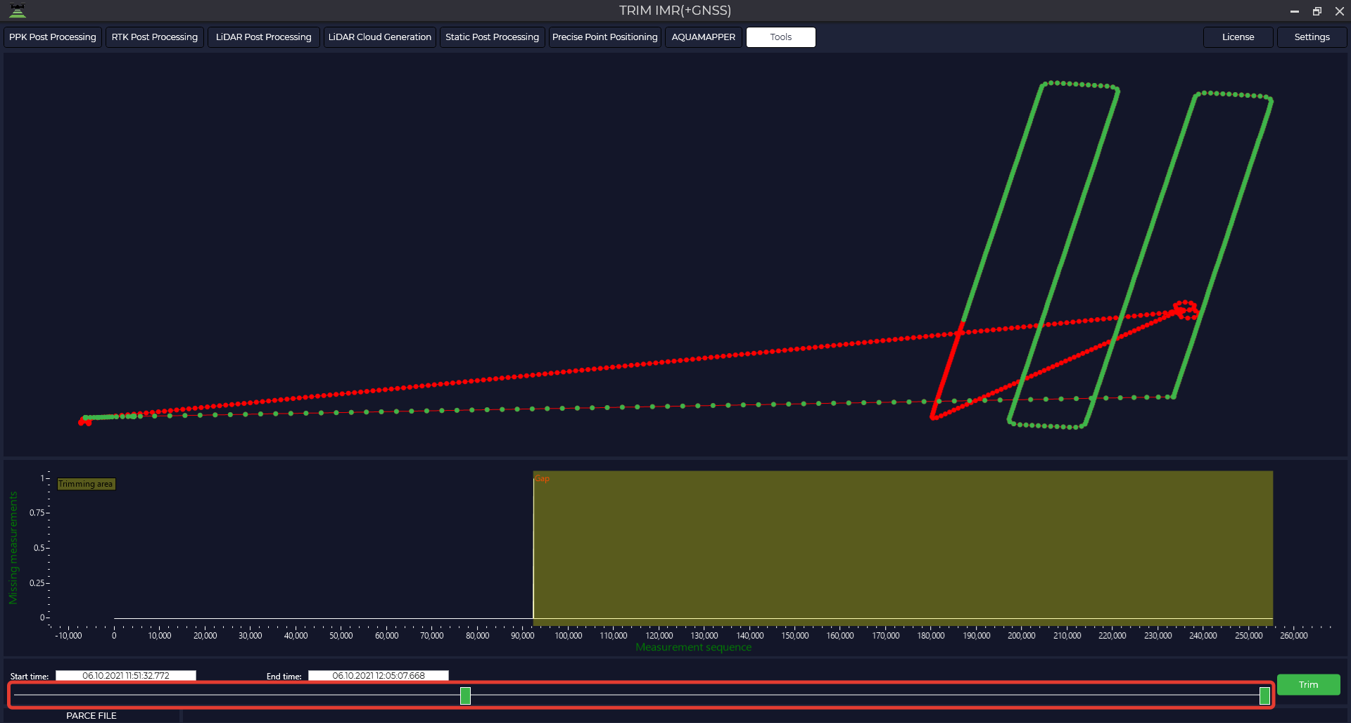
After selecting the desired segment using the sliders at the bottom of the screen, click "Crop". The IMU file will be saved to the folder in its original format at the interval you specified and will be saved to the original folder.
Trim IMR
To eliminate jumps in inertial navigation unit (IMU) data when performing work without satellite navigation data, you can use the IMR Trim tool.
This tool is useful if the dataset contains an error message - IMU file contains gaps in measurement points! Use the IMR Trim tool to remove the missing sample time interval.
To start the tool, select IMR Trim in the Tools, Trim/Stitch tab. Then select the file in *.imr format to be trimmed.
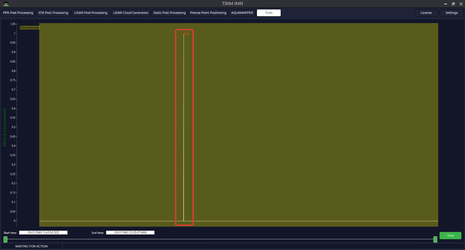
For further correct processing it is necessary to exclude omissions from the data, therefore the IMU file should be divided into two segments and further processed in two parts. Only one segment is trimmed, so in this case we need to repeat this procedure twice.
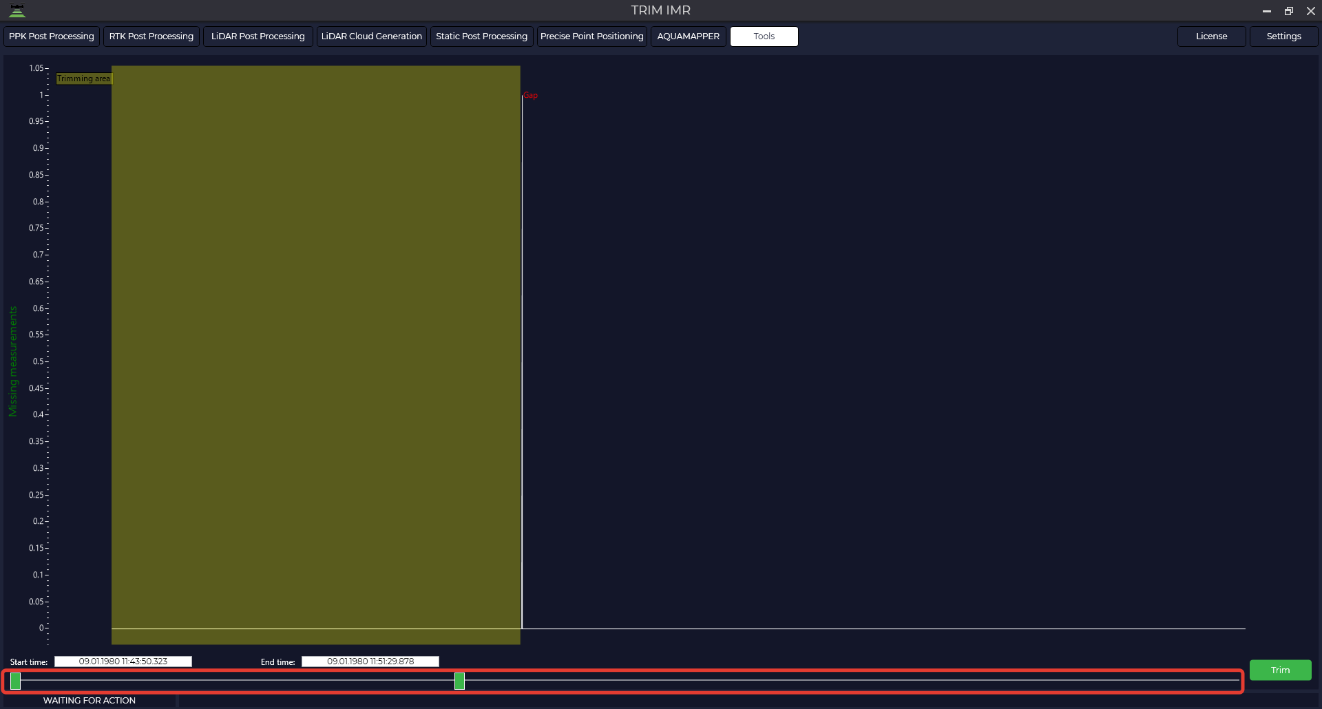
After selecting the desired segment using the sliders at the bottom of the screen, click "Crop". The IMU file will be saved to the folder in its original format at the interval you specified and will be saved to the original folder.
Coordinate converter(One coordinate)
This tool allows to convert data from WGS-84 coordinate system to another one using *.prj file of coordinate system, which is loaded into the program database or using calibration file, which was made before in TOPODRONE Post Processing program. For more details see Calibration.
For example, this tool can help you to convert a base station coordinate from local coordinate system to WGS-84 when processing an area in the LiDAR Post Processing module.
In order to convert one point from WGS-84 coordinate system to any other, you should choose Coordinate Converter in the Tools tab, then One coordinate.
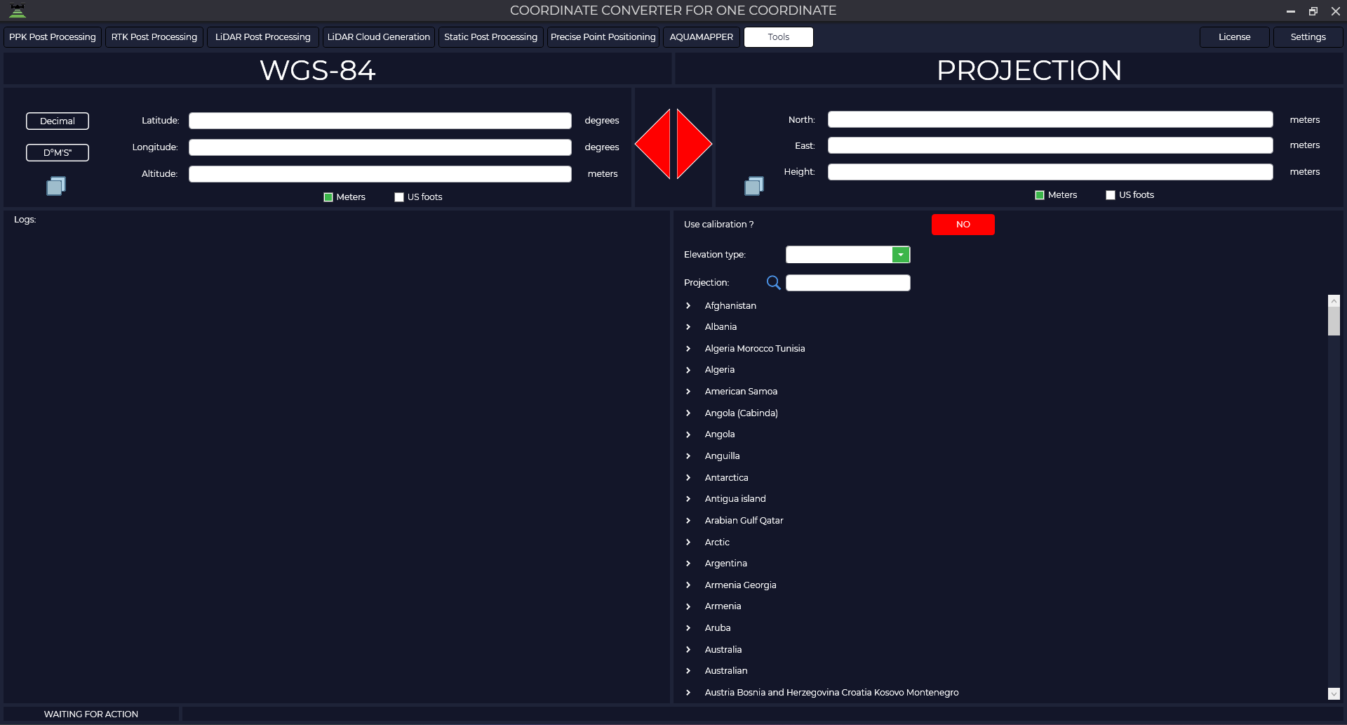
Select the coordinate format (decimal or degrees, minutes, seconds)

Next, select the desired height type.

Select the required coordinate system. The required *.prj file can be quickly found using the search bar. The coordinates of the source point must be within the area covered by the *.prj file.

If you have calibrated in the TOPODRONE Post Processing program, press the "NO" button and select your calibration file.
After that, click on the right arrow, which will change its color to green when you hover your mouse cursor over it. Click on the arrow with the left mouse button.

After that, the converted coordinate values of the source point in meters will appear in the right part.

Coordinate Converter(Coordinates from file)
The tool allows you to convert coordinates from one coordinate system to another using the *.prj coordinate system file loaded into the program database or the calibration file created earlier in the TOPODRONE Post Processing program. More details about this process can be found in the "Calibration" section. To convert a coordinate catalog from one coordinate system to another, go to the "Tools" menu and select "Coordinate Converter", then "Coordinates from file".
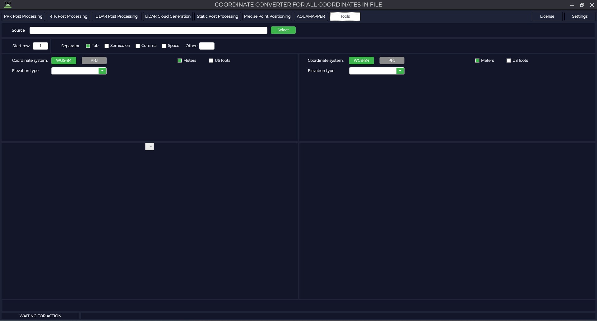
In the Source section, specify the coordinate catalog file you want to convert, the import start line, and the coordinate separator type.

Select the coordinate system and elevation type of the original coordinate catalog.

Determine whether the columns match the values.

Specify the coordinate system and elevation type of the target coordinate catalog.

If you have calibrated in the TOPODRONE Post Processing program, press the "PRJ" button, then press "NO" and select your calibration file.
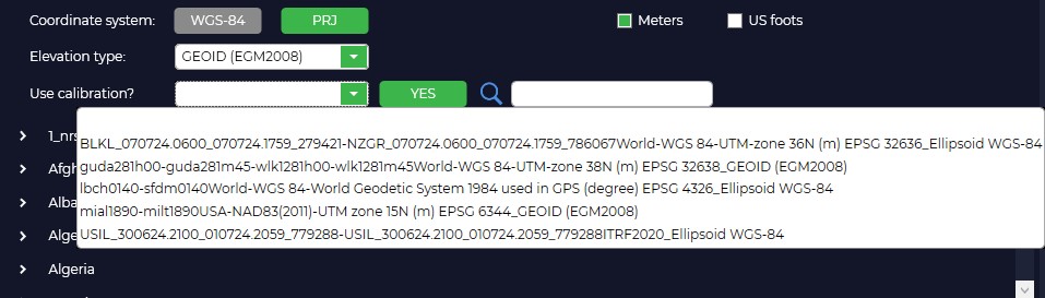
After pressing the "Start" button, the right window will display the coordinate catalog in the selected coordinate system. If necessary, click the "Save" button and save the new file.
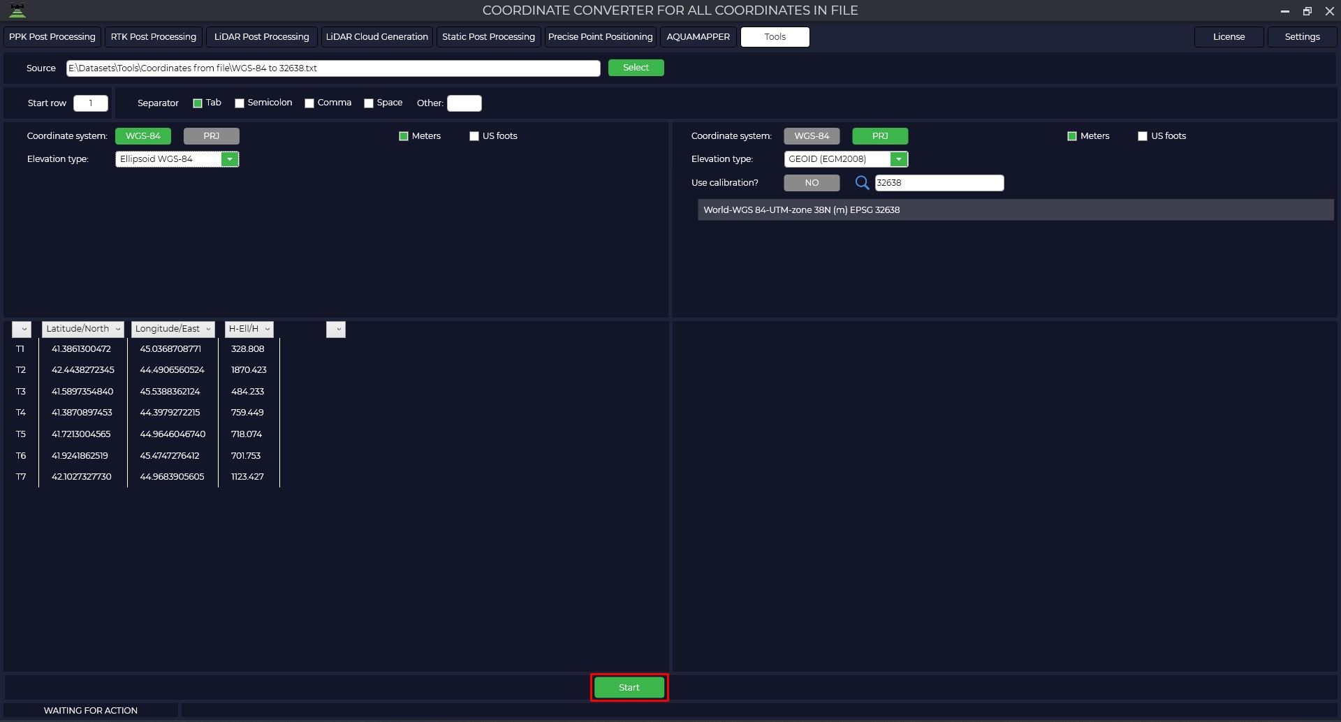

Maps
The "Maps" module is designed to display loaded static observations and vectors at all stages of data processing. To launch the module, go to the "Tools" tab and click the "Maps" button. Important: for correct display of observation points, the map window should be opened when loading files. If this condition has not been met, you should re-download the data. An additional function of the module is to measure the distance between two points on the map. To do this, press the "Ctrl" key and select two points in the map area with the left mouse button. The value of the measured distance will be displayed in the log window.
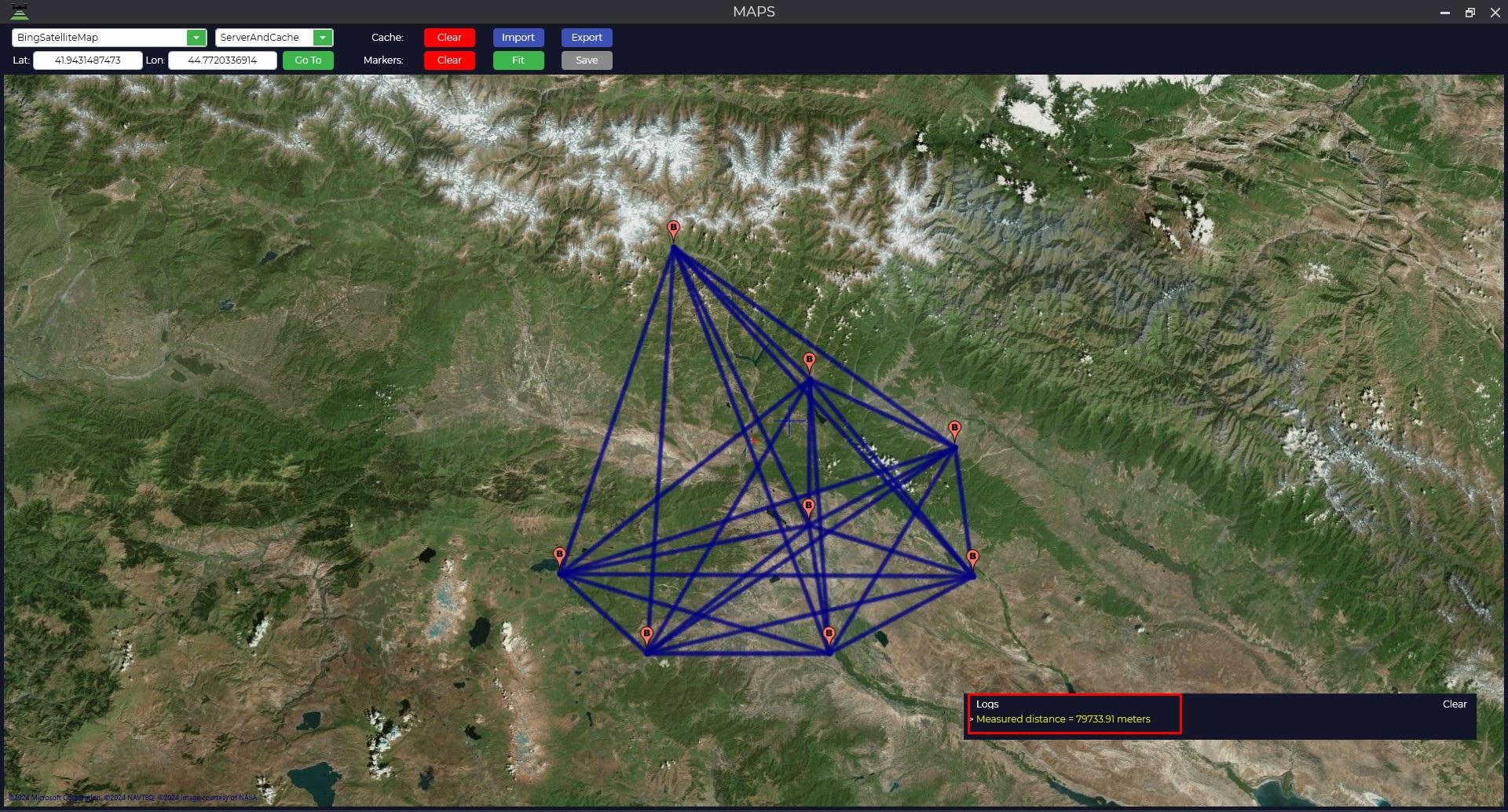
GNSS data converter
The module is based on the open source software RTKLIB, this module is designed to convert raw observation files from Global Navigation Satellite System (GNSS) receivers into RINEX format. The module supports data formats from the following GNSS chip manufacturers: U-blox, ComNav, NovAtel, Hemisphere, Javad, Trimble, as well as the common *.YYO format, where YY is the year of observations.
To convert data to *.obs format, perform the following actions: Go to the "Tools" tab and select "GNSS Data Converter" in the RINEX section. Specify the file to be converted to *.obs format.
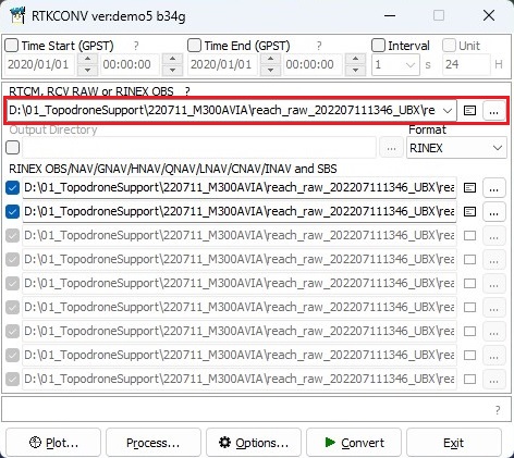
The lower part of the window displays the files to be exported.
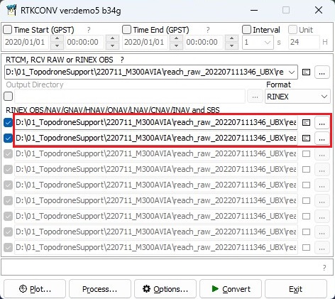
If necessary, time-limit the file by specifying the date and range of operation, and change the frequency of the final file write.
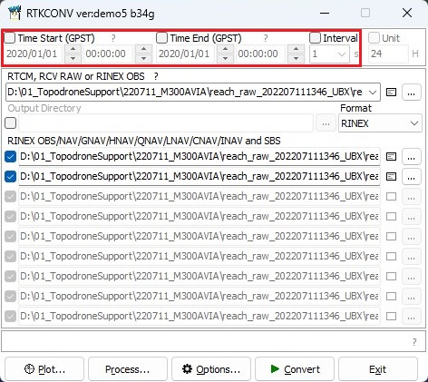
Click on the "Options..." button and select the RINEX version, satellite constellations, operating frequency or specific satellites. Then click on the "OK" button.
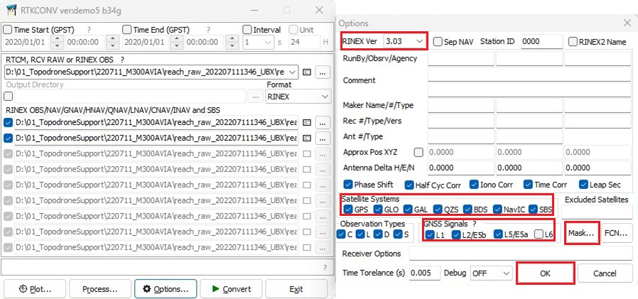
Click on the "Convert" button to have the program convert your file to RINEX format with your parameters.
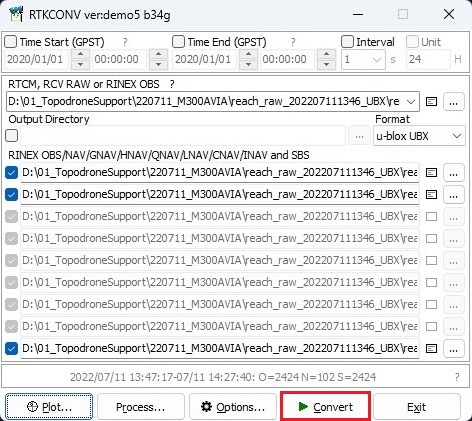
After converting the file, click on the "Plot..." button to evaluate the quality of your data. For more information about data quality analysis, see Appendix B.


RINEX merger
This function is designed to merge measurement files received from different receivers of the global navigation satellite system into one file. It is especially useful when the reference base station provider divides files into time slots when downloading data.
Follow the steps below to merge the files: Go to the Tools tab and select Merge under RINEX.
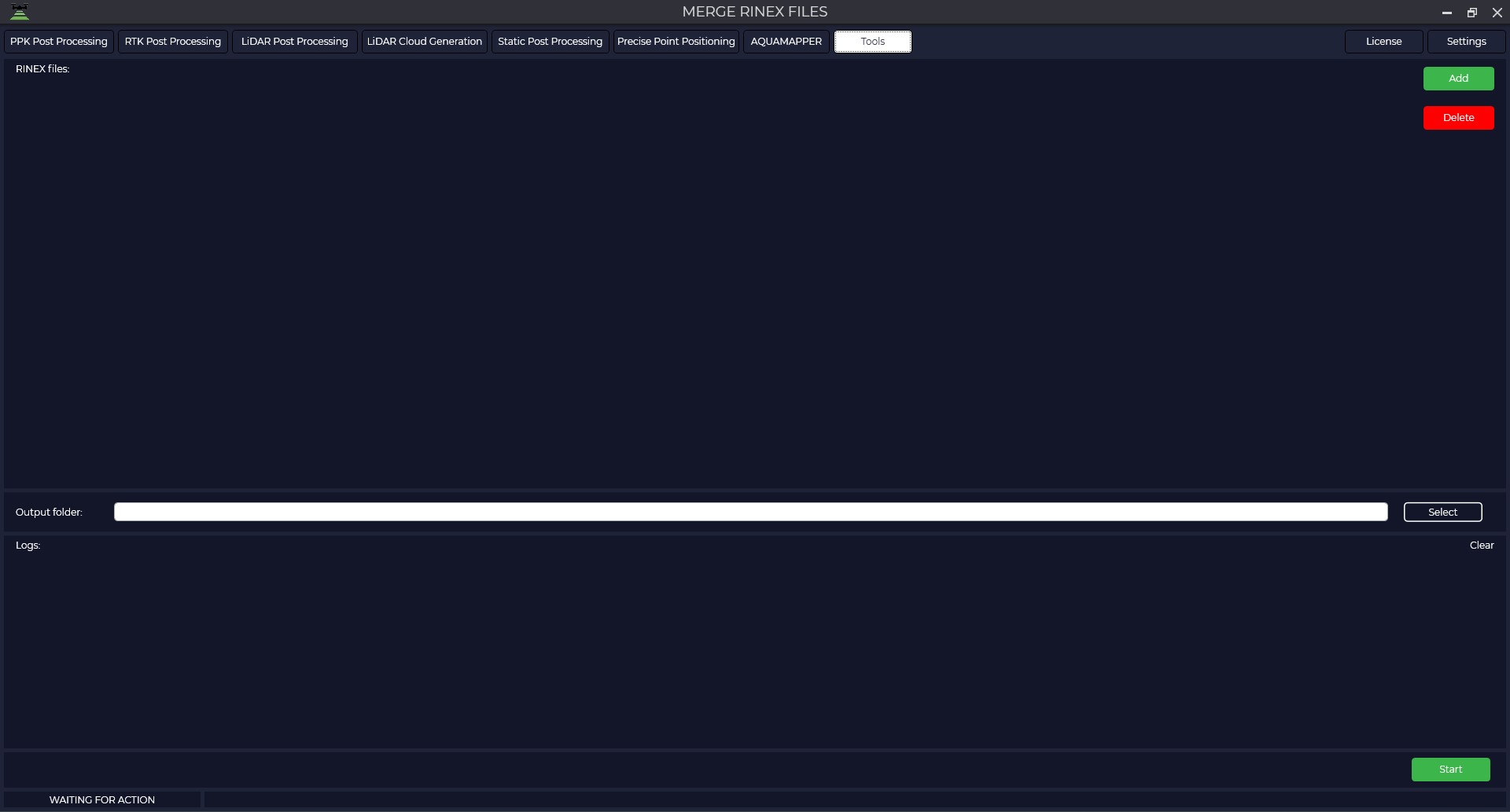 Click the "Add" button to add measurement files and select the required files in *.rnx, *.**o and *.obs formats.
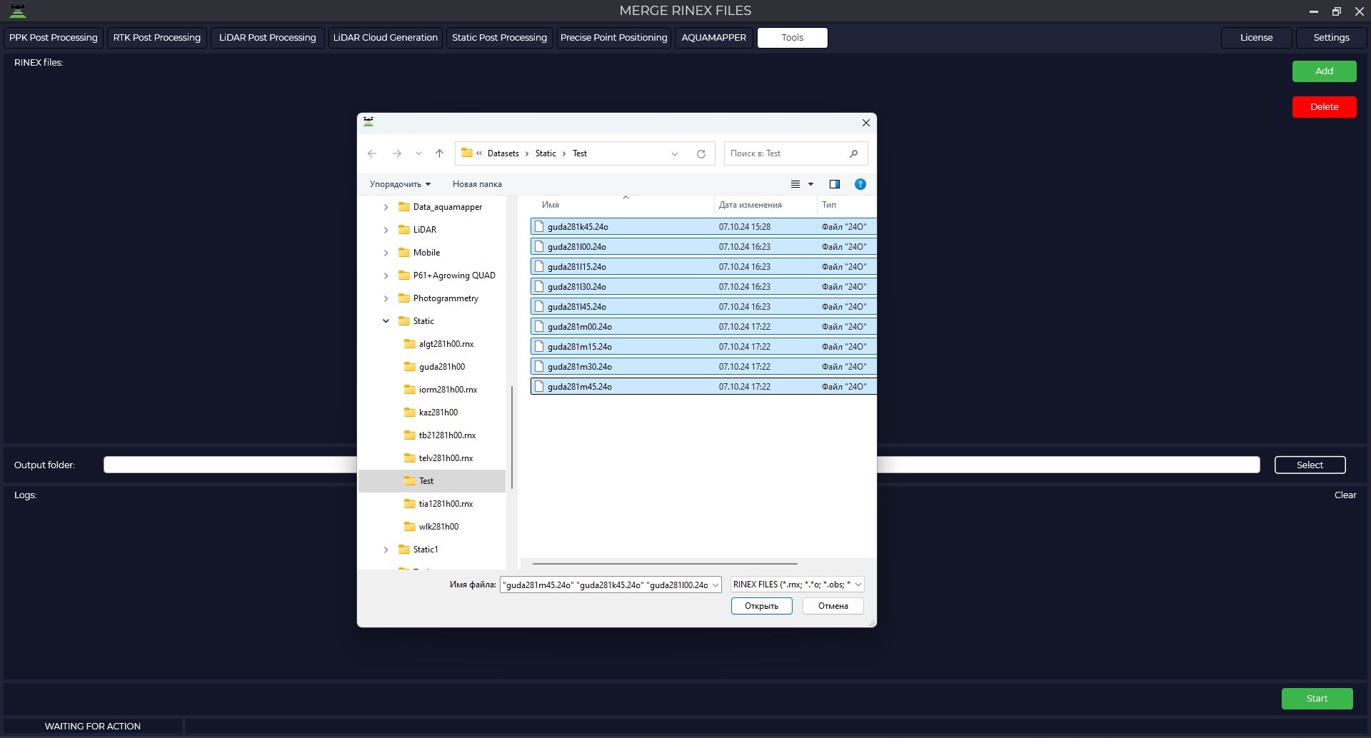 The "RINEX files" window will display the downloaded files, and the "Logs" window will display information about the recording time, antenna type, and receiver coordinates that the program reads from your files.
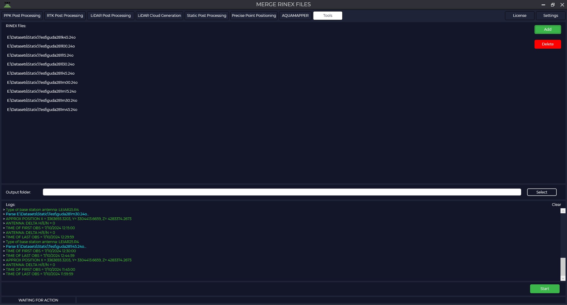 Specify the path to the folder where you want to save the merged file.
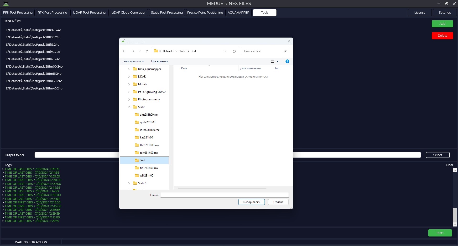 Click on the "Start" button to have the program merge all files and save to the previously specified folder.
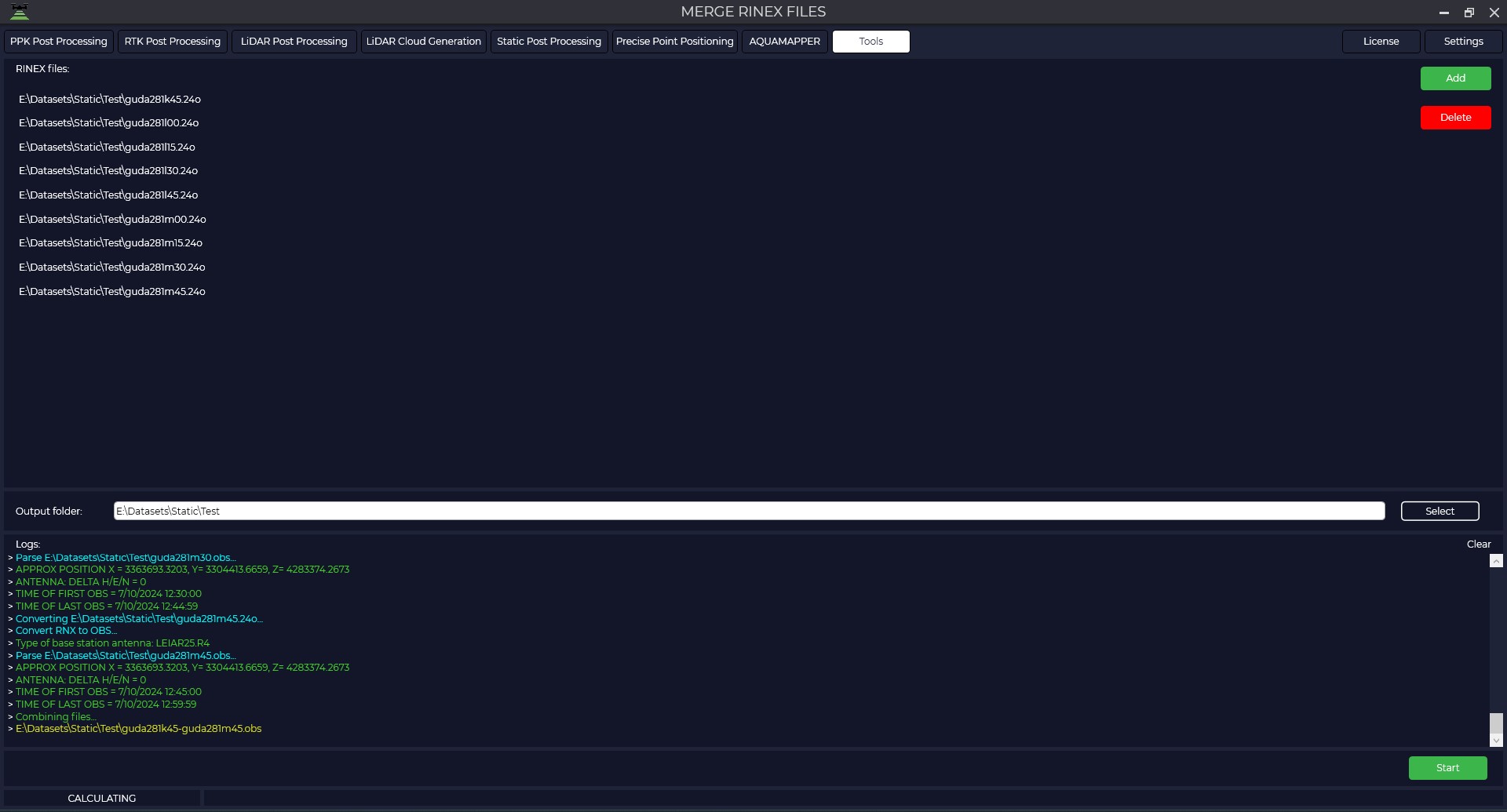 After the file merge operation is successfully completed, you can use the resulting file for further data processing.
Satellite filtering
This module allows you to exclude certain satellite constellations or specific satellites from the observation file, which may be necessary to improve data quality.
Follow the steps below to filter satellites: Go to the "Tools" tab and select "Rinex", then "Satellite Filtering".
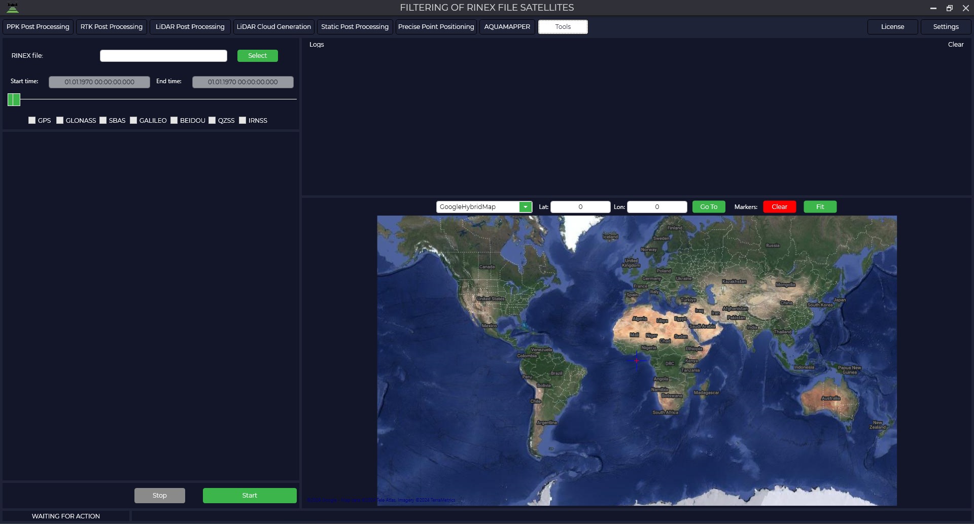
In the upper left part of the RINEX file window click the "Select" button and specify the raw observations file in *.obs format.
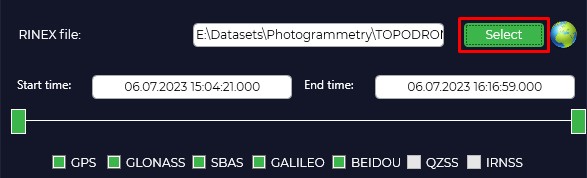
Click on the icon to view the signal quality  to open the "Plot" window, which allows you to understand which satellites may be interfering with data processing. For more information about data quality analysis, see Appendix B.
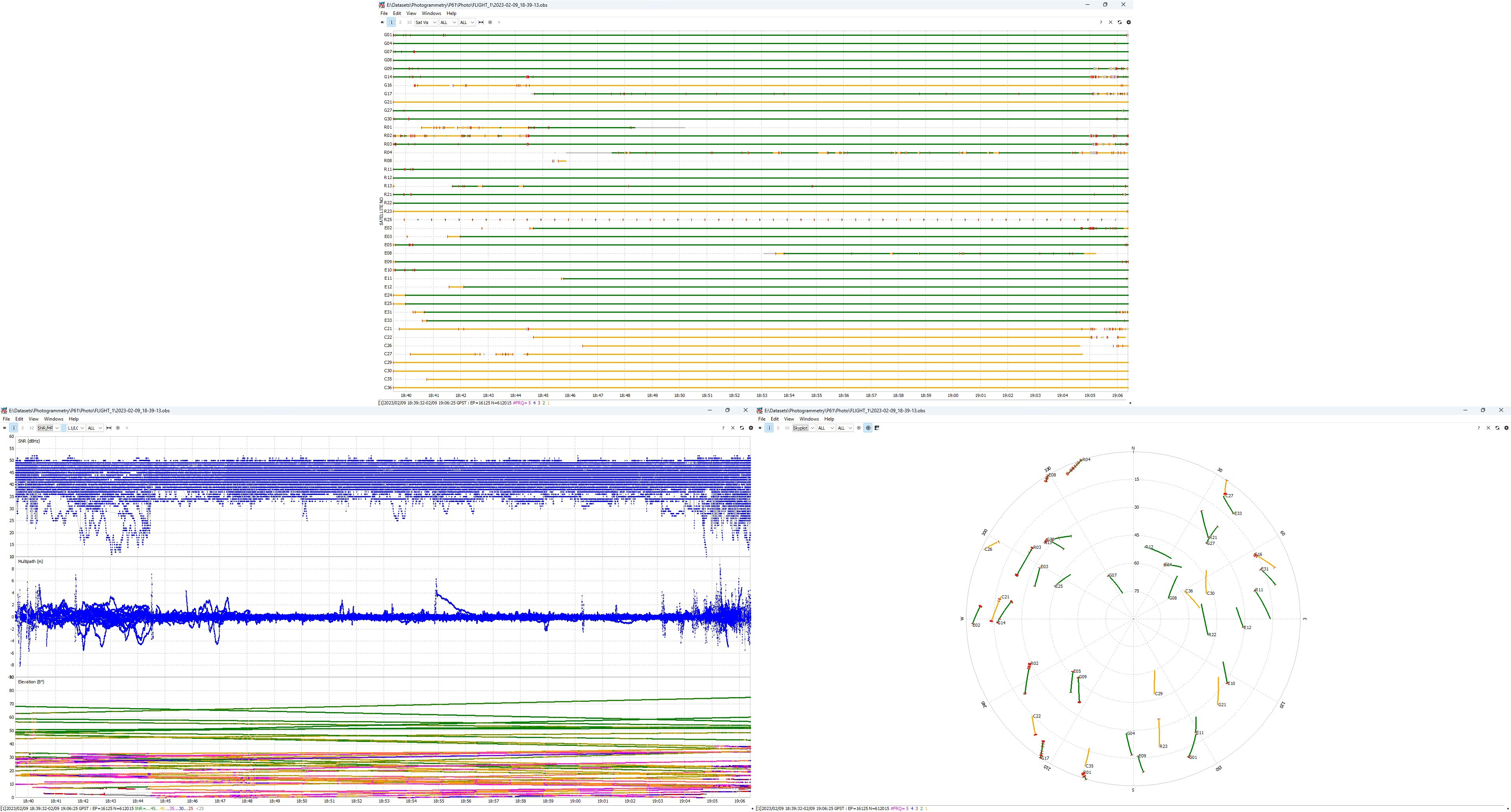
Move the sliders left and right if necessary to change the start and end time of the file.
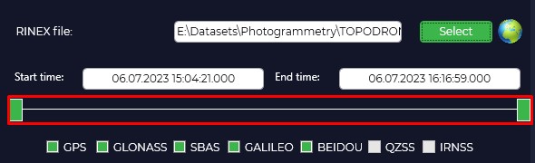
Uncheck the required checkboxes if you want to exclude certain satellite constellations (GPS, GLONASS, GALILEO and BEIDOU) or specific satellites.
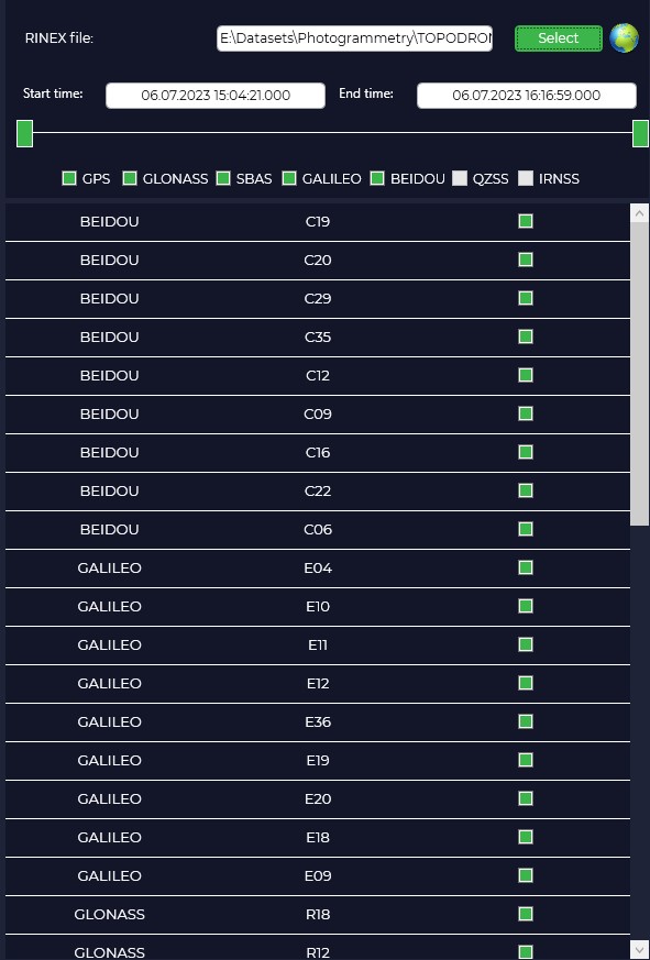
Press the "Start" button. The program will save the new file, excluding the selected satellites from it.
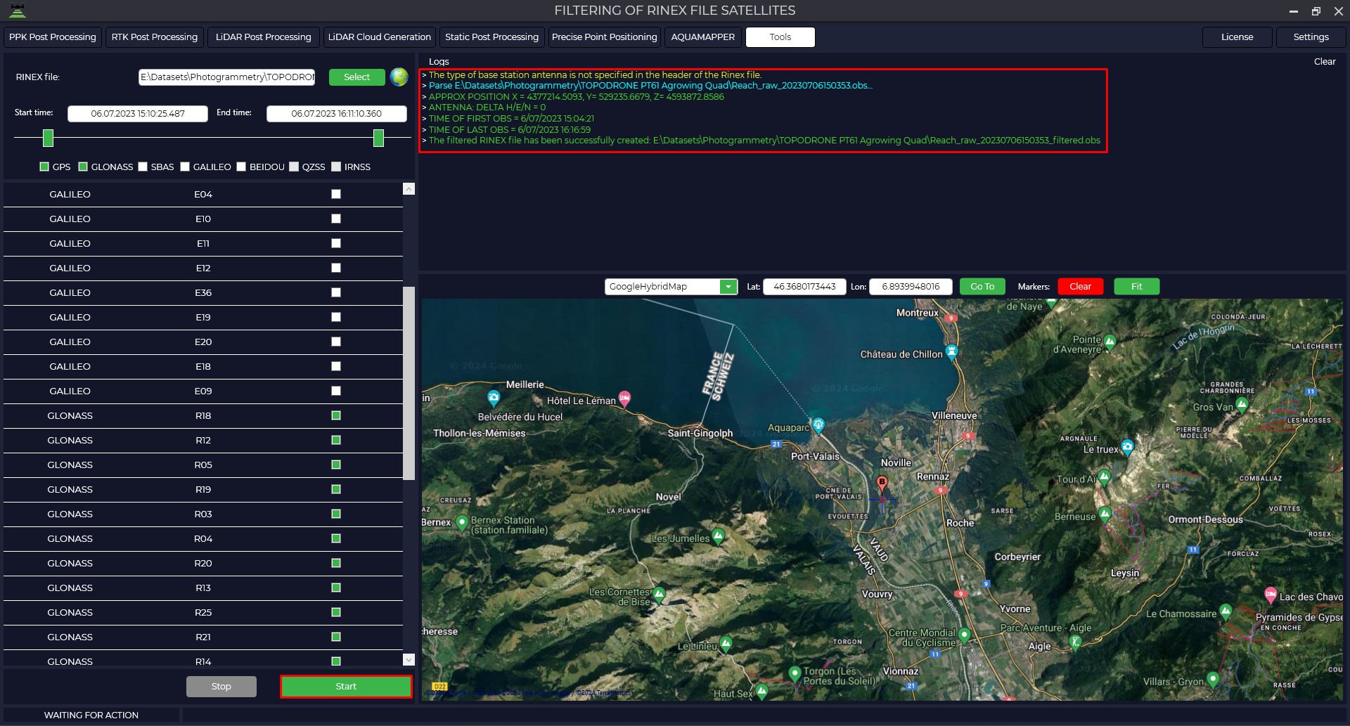
Once the satellite filtering operation has been successfully completed, you can use the resulting file for further data processing.
Calculating the focal length
This tool is not directly related to GNSS data processing, but it helps to calculate the focal length of the camera, which is necessary for data processing in photogrammetric programs.
Instructions for calculating the focal length:
1. Click the Tools tab and select Focal Length Calculation.
2. In the opened window specify the following parameters: flight altitude of your aircraft, previously obtained focal distance in millimeters (from the result of aerotriangulation in photogrammetric software) and error values by height of your control points.
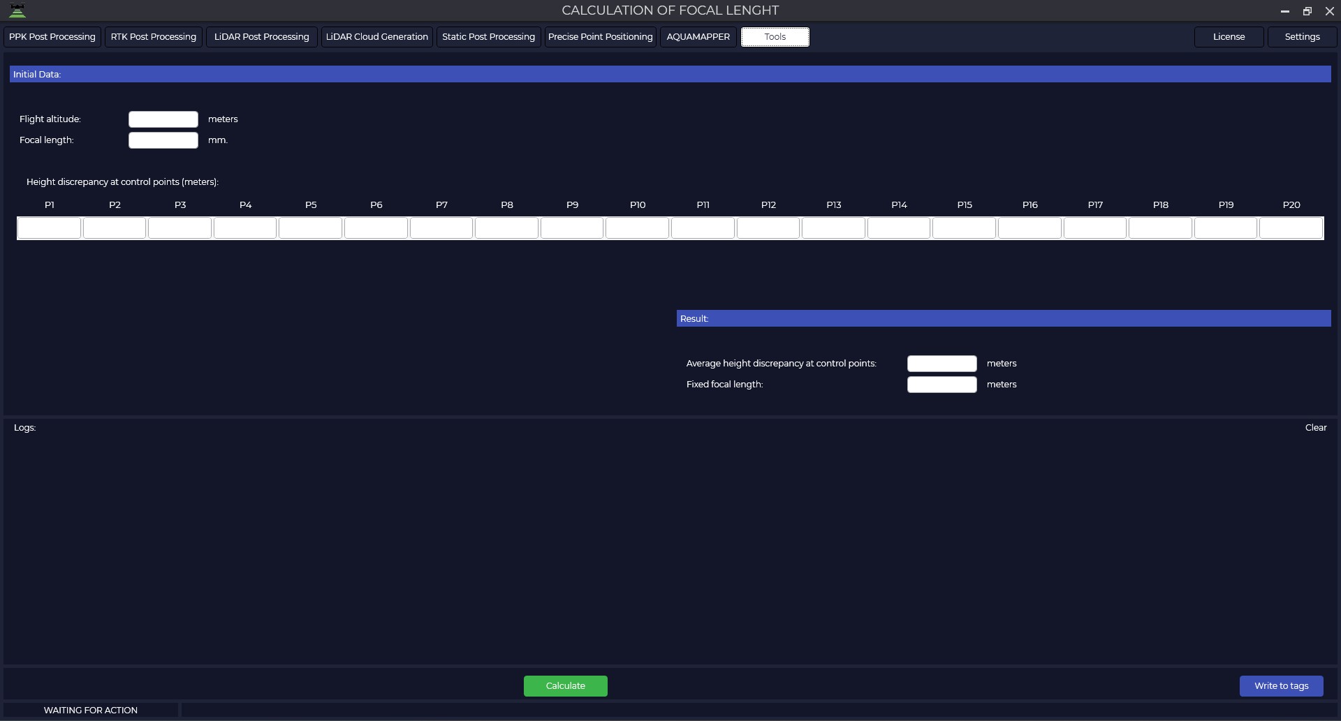
3. Click the "Calculate" button. The program will calculate average height error and focal length, which can be used in photogrammetric programs.
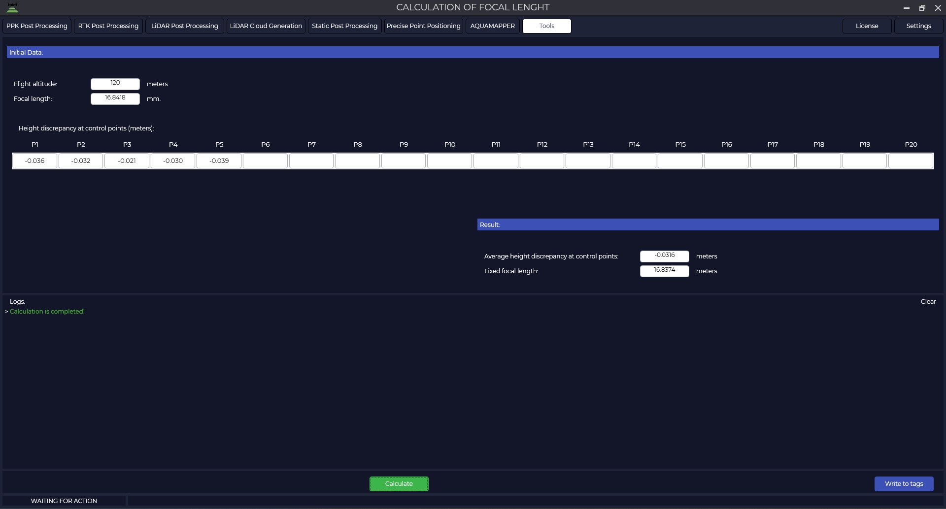
4. If necessary, the new focal length can be written to the EXIF tags of your photos by clicking the "Write to Tags" button. This will help in further photogrammetric data processing.
5. Specify the folder with the photos.
6. The program will write the new focal length to all photos in the specified folder.
The program replaces the focal length in the original files without creating copies of the photos.

Settings
General
In the general settings of the TOPODRONE Post Processing program, you can perform the following actions:
Change the language of the program interface and output logs during processing.

In the "Geoids" window you can add or remove the type of geoid to be used in postprocessing. If necessary, you can import another geoid in *.gtx format. To do this, click the "Add" button and select the required file.
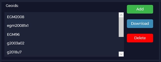
If necessary, you can delete a geoid model from the list by clicking the "Delete" button.
It is also possible to download a geoid model from the server. To do this, click the "Download" button, find the required geoid model and click the "Download" button.
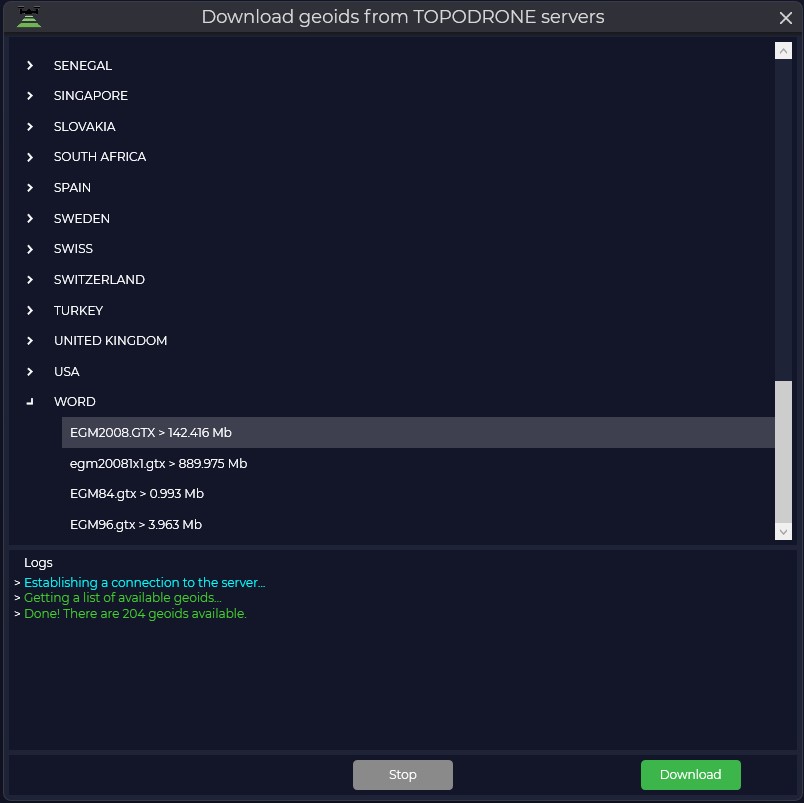
The "PRJ" window displays a list of available coordinate systems that will be available for selection during postprocessing.
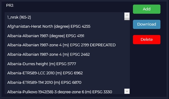
You can add or remove the required coordinate system from the list. To add a coordinate system, click the "Add" button and select the desired file. Files in *.prj formats are supported, other coordinate system formats are not supported.
If it is necessary to delete a coordinate system from the list, click the "Delete" button. Complete deletion of imported coordinate systems is possible only after program restart. The "Calibrations" menu displays available calibration parameters, which are used for transition from one coordinate system to another.
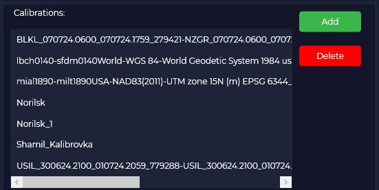
By default, several calibration files are added for some zones. To add a calibration parameter, click the "Calibrations" button and select the desired file. Files in *.tpc format are supported, other coordinate system formats are not supported.
Aerial photography
Select the Aerial Photography tab to customize the processing parameters of the PPK Post Processing and RTK Post Processing modules.
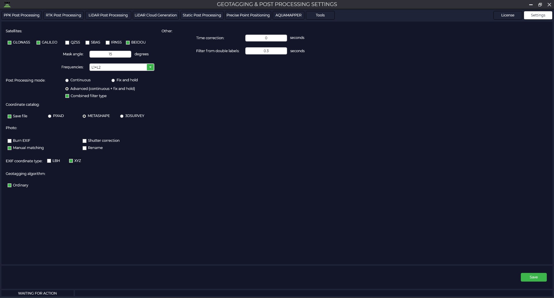
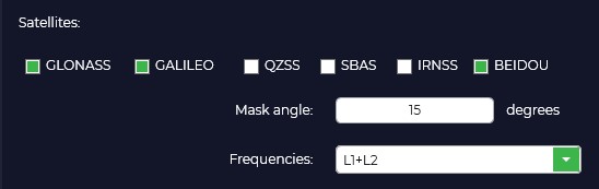
In the Postprocessing Mode window, you can select from Continuous, Fix and hold, or Advanced.

In "Fix and Hold" mode, the program strives to obtain a fixed positioning solution that provides the highest accuracy and reliability. It uses information from the base station and rover to calculate the relative position and then amplifies this solution to achieve a fix. When a fix is achieved, the program holds this solution for as long as possible, even if the signal quality temporarily drops or some satellites are lost.
The purpose of the "Fix and Hold" mode is to provide a stable and reliable fixed solution, which is particularly useful in surveying applications where high accuracy and long-term stability are required. This mode may be preferred when it is important to avoid switching between solutions and to ensure continuity of the fix even in the face of temporal changes (e.g. signal reflections or passing through obstacles).
In "Continuous" mode the algorithm processes data continuously and updates positioning results as new data is received. In contrast to the "Fix and Hold" mode, here the program does not fix the solution, but continuously calculates the rover position based on the current data. When new observations are received, the program updates the position taking into account these data and previous results.
Continuous mode provides more relevant positioning results because it continuously updates the position based on the latest data. It can be useful in applications where relevance and dynamic position changes are more important.
The choice between "Fix and Hold" and "Continuous" modes depends on the specific requirements and conditions of the application. If stability and reliability of solution fixation is important, especially under static conditions, the "Fix and Hold" mode may be preferred. If relevance and dynamic positioning are more important, "Continuous" mode provides a more continuous position update based on the latest data.
The "Advanced" mode is a combination of the previous modes with all their pluses, but data processing takes a little longer.
In the "Coordinate Catalog" window, you should check the "Write File" box to save the catalog of photo centers and select the file format for the program you are using.

In the "Photos" window you can save the coordinates of the photo centers in the EXIF file of the photo, assign a unique name to the photos depending on the time of creation, it is recommended to check the "Manual matching" checkbox for correct matching of photos and marks, the "Shutter correction" checkbox is responsible for shifting the mark by half the shutter time.
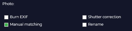
In case you checked "Write tags" in the previous window, you should select the format of coordinates saving (LBH - geographic coordinates, XYZ - rectangular coordinates).

The "Geotagging Algorithm" tab contains settings to help the program match photos and tags in the event of a quantity mismatch.
Normal - the alignment is done in the order of the photos taken.
Increase time weighting - matching is based on the time the photos and tags were created.
Increase coordinates weight - Matching is performed by navigation coordinates of photos contained in tags and high-precision coordinates of tags as a result of post-processing in TOPODRONE Post Processing program.
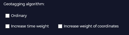
In case of routes where some photos are overlapped with other photos, the coordinate matching algorithm may not work correctly. Example: route on one battery when shooting a small object for 3D reconstruction. In the case of shooting when the camera is pointing at nadir and then immediately shooting when the aircraft is shooting perspective.
The double-tag filter allows you to remove unnecessary tags at the post-processing stage. Default value 0.2 seconds.

Lidar scanning
In this section of the program you can configure parameters for high-precision trajectory processing, point cloud generation including TOPOSLAM technology.
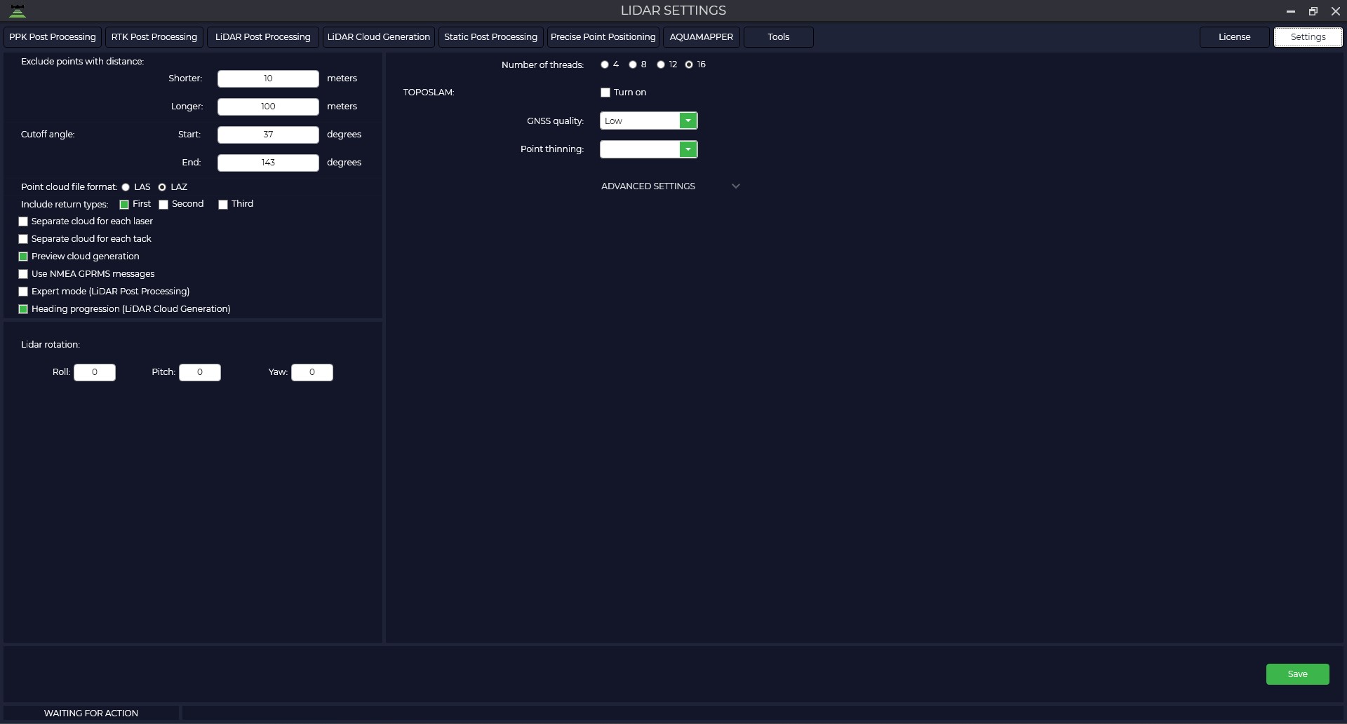
|
|
Exclude points with distance from lidar Closer is the distance to disregard when generating the point cloud. Cut angle: Specify the start and end angle of the LiDAR scan. Include return types in the point cloud - select the number of reflections you need or the number that your hardware supports. Preview cloud generation - view point cloud generation in real time |
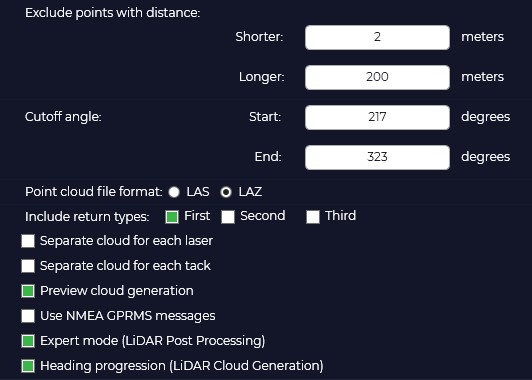
Synchronize time by NMEA GPRMC packets -
Expert mode (LiDAR Post Processing) is a mode that allows you to manually specify the type of sensor and IMU to be used.
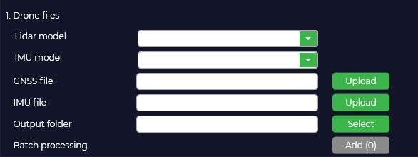
TOPOSLAM is designed to correct the point cloud when the GPS signal is not good enough. Currently TOPOSLAM only supports ground scanning.
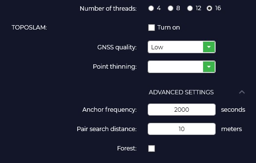
Number of streams. Specify the number of processor threads you would like to utilize to accelerate SLAM processing.
To activate the TOPOSLAM algorithm, you must check the corresponding "Enable" option.
GPS signal quality. Depending on the quality of GPS track you should select the appropriate tab. Low - floating solution more than 70%, Medium - floating solution more than 50%, High - floating solution more than 20%. If the quality is low, the program splits the track into smaller segments for their further mutual comparison.
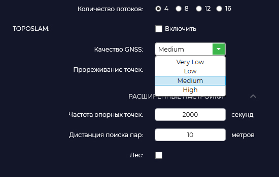
Point thinning. Segment skipping function. Off - do not skip, Low - skip one segment after each generated segment, Medium - skip two segments, High - skip four segments. This function is designed to speed up the processing process and in case of RAM shortage for large shootings.
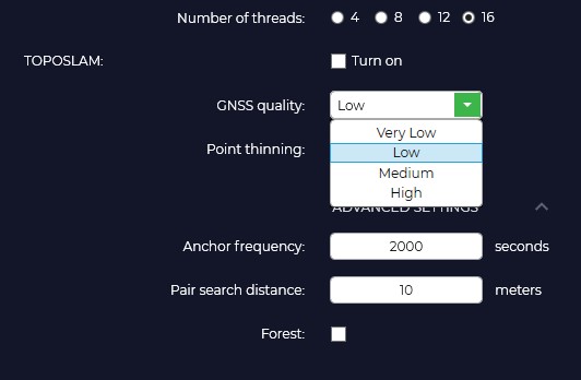
Frequency of reference points.
Distance search for pairs.
Forest.
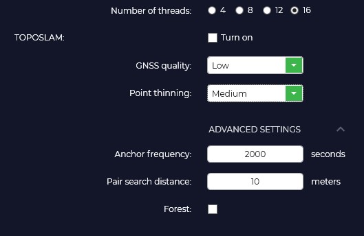
Laser scanner track file structure
To customize the track file structure, go to the Settings tab, then select Lidar Scanning and select the Track File Structure option from the drop-down list. In the opened window you should specify the trajectory file obtained as a result of postprocessing.
If you have performed processing in TOPODRONE Post Processing software, specify the order of the columns according to the following example:
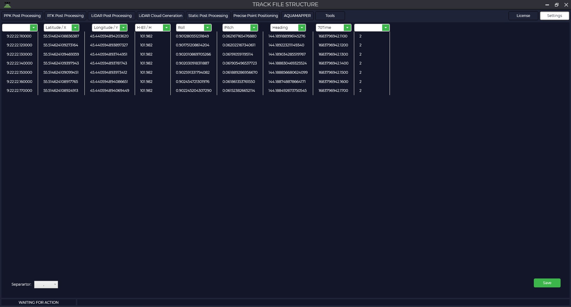
After filling in all the fields, click the "Save" button.
This procedure only needs to be performed once. If you continue to use the TOPODRONE Post Processing software, you will no longer need to specify the track file structure. However, if you have been processing in any other software, the structure of the track file will be different and you will need to specify the appropriate field order for your track file.
Laser Scanner Sensor Beam Calibration
To set the laser scanner sensor beam calibration, go to the Settings tab, then select Lidar Scanning and select the Lidar Calibration option from the drop-down list. Then select the model of your laser scanner.
In the window that opens, you will be able to turn off unnecessary beams or adjust the necessary calibration values.
Important Note: Laser scanners manufactured by TOPODRONE are factory calibrated and do not require recalibration during their entire lifetime.
|
|
Use – beam number
The number of lidar beams depends on the model of your laser scanner and may vary depending on the type of device. |
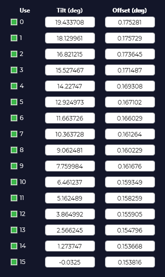
AQUAMAPPER
Select the "AQUAMAPPER" tab to configure the processing parameters of AQUAMAPPER modules.
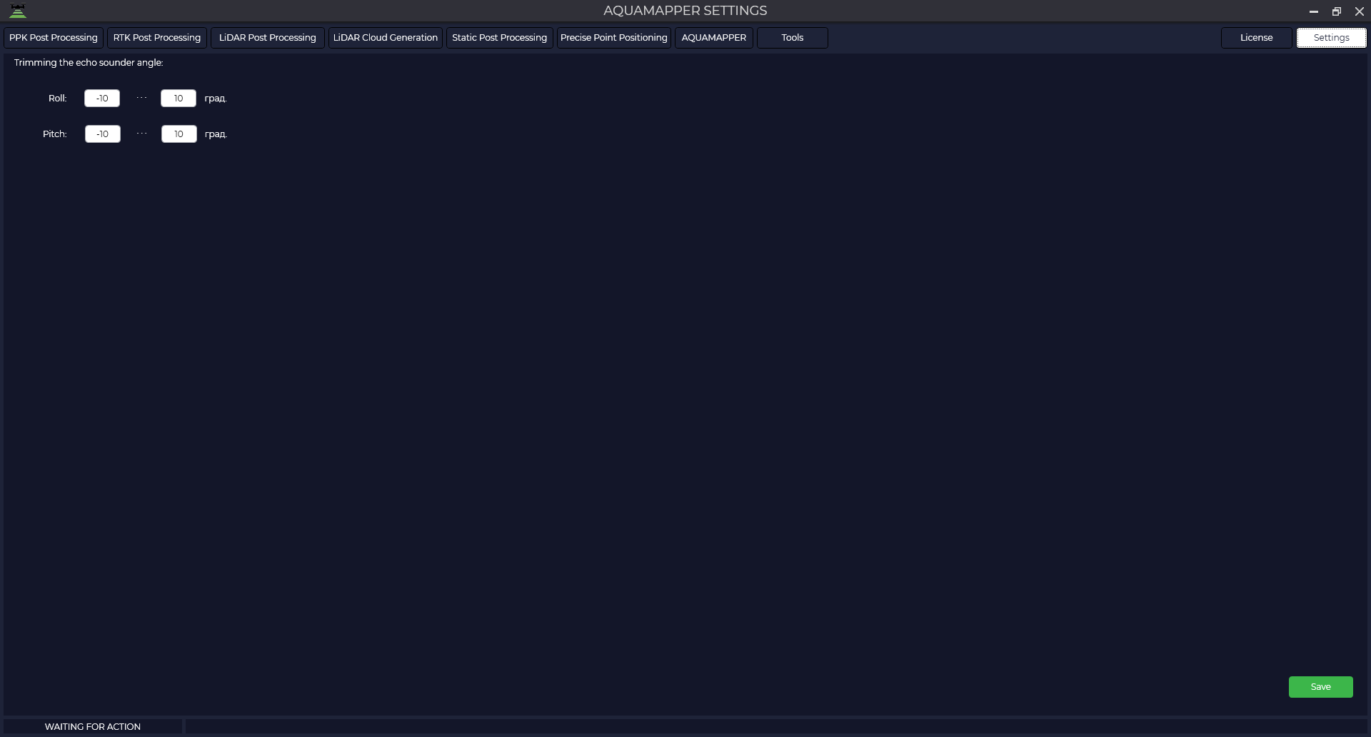
If necessary, adjust the Roll and Pitch angles. Closer to zero values of these angles will help to increase the share of vertical measurements in the processing process.
The optimal angle values are in the range from -8 to +8 degrees.
Appendix A. Manual matching of photographs and timestamps.
In some cases, the number of photographs does not match the number of time stamps collected during aerial photography. To solve this problem, the TOPODRONE Post Processing program provides an algorithm for manual matching of photos and time stamps.
To activate this mode, you need to check "Manual matching" in the aerial photo settings.
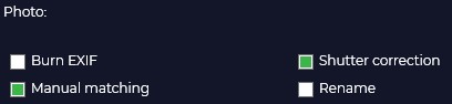
The "Geotagging Algorithm" tab contains parameters that help the program match photos and tags in case of quantity mismatch. There are three options for matching:
- Normal: The photos are combined in the order in which they are taken.
- Increase time weighting: the matching is done by the time the photos and tags were created.
- Increase coordinate weighting: matching is based on navigation coordinates contained in photo tags and high-precision label coordinates resulting from post-processing.
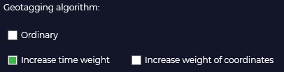
During processing, the program displays information about the number of timestamps and the number of snapshots in the "Logs" window.
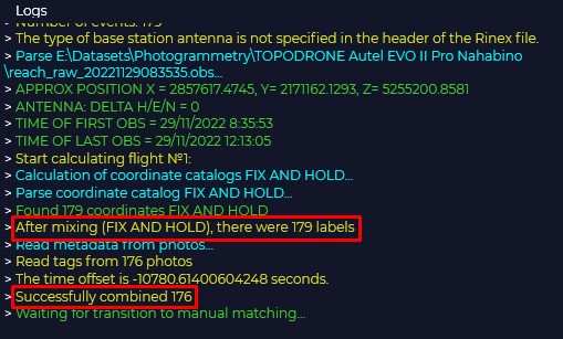
If the number of labels and images do not match, an additional window appears with information about the number of images, coordinates in the catalog and the number of matches.If you need to perform manual matching, you should answer "Yes" to the program's question "Match manually?".
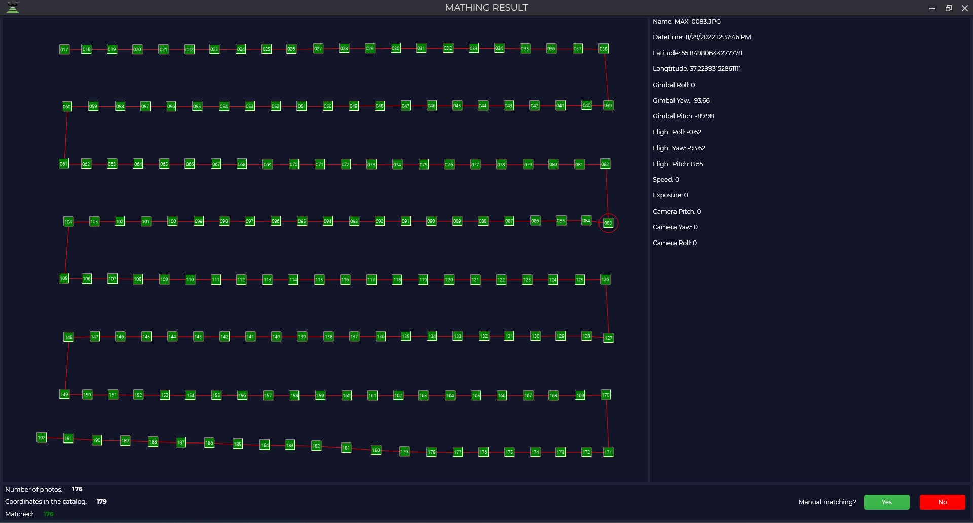
Then in the next window, the left side contains information about the photos and the right side contains coordinates. The upper part of the data is presented in tabular form, the lower part - in graphical form.
If your dataset has no navigational coordinates, the left side of the window will remain blank.
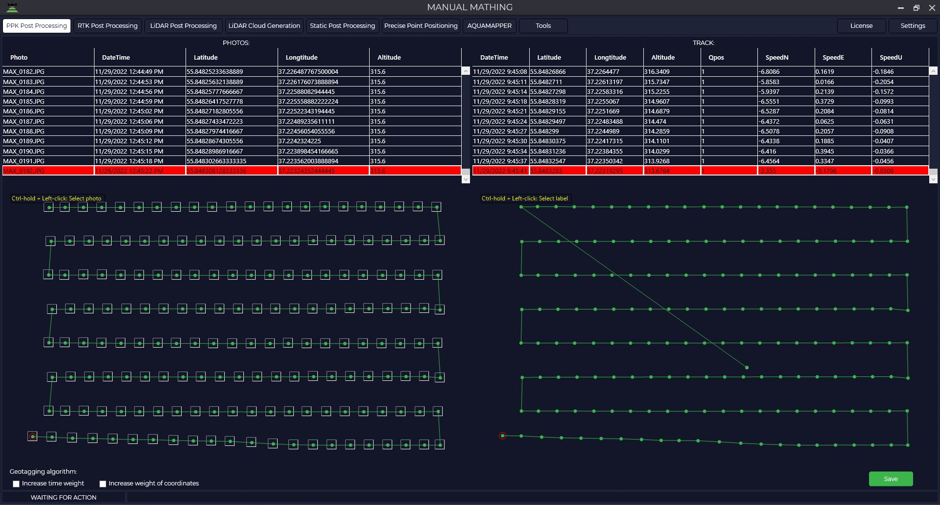
To perform a match, you need to select a photo and its corresponding label with the left mouse button while holding down the CTRL key, and then click the "Save" button.
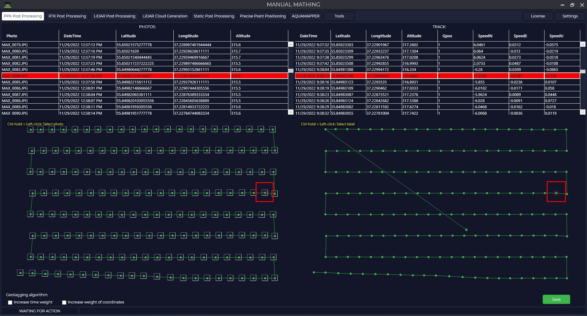
If the matching is successful, you must answer the program's question "Match manually?" with "No".
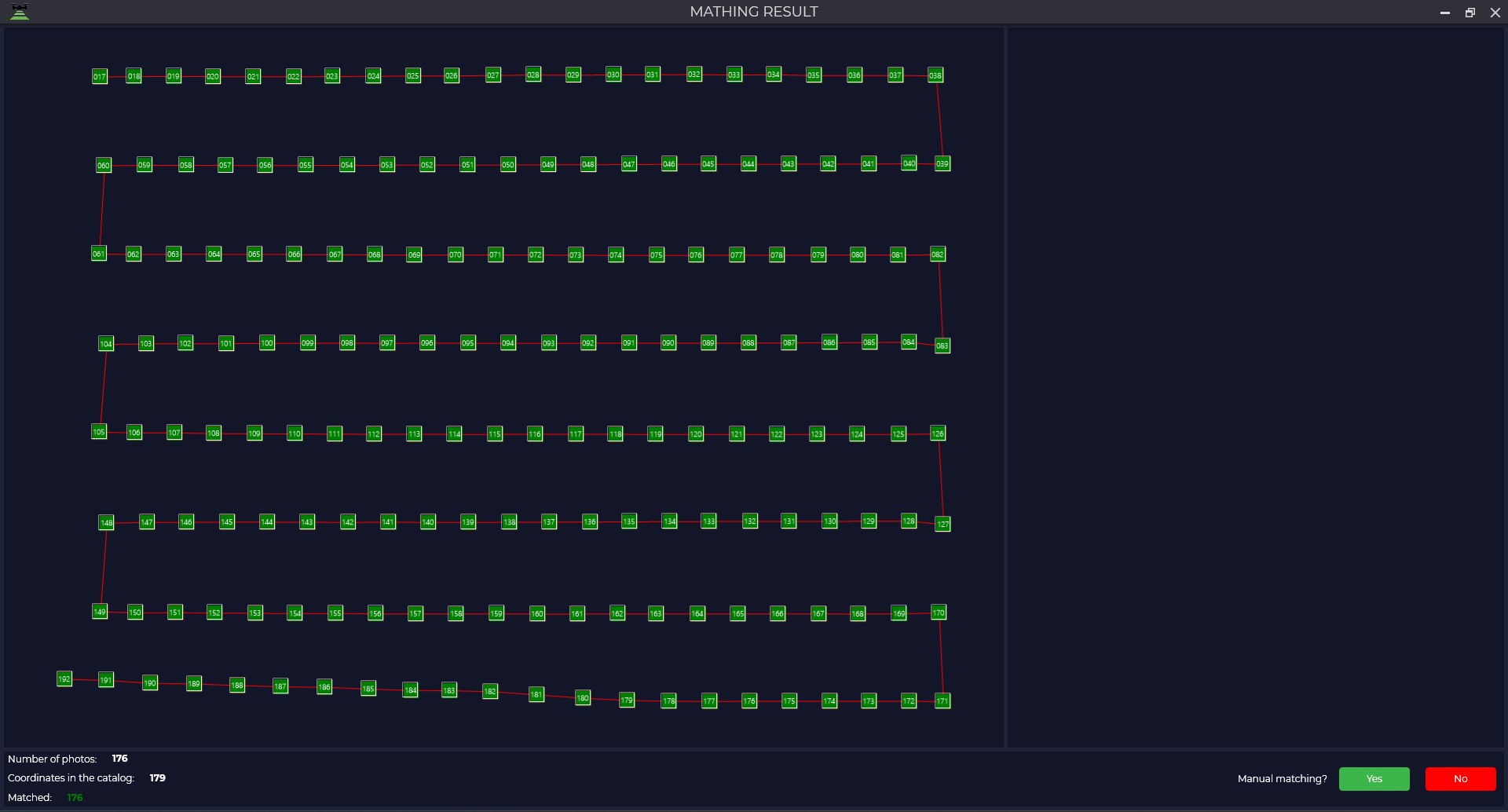
The program will form a catalog of photo centers and you can proceed to photogrammetric processing.
Appendix B. Analysis of GNSS data.
During GNSS data processing, it is essential to monitor satellite availability, their spatial distribution, and the quality of received signals. Specialized visualization tools are used for this purpose, each providing data for analysis.
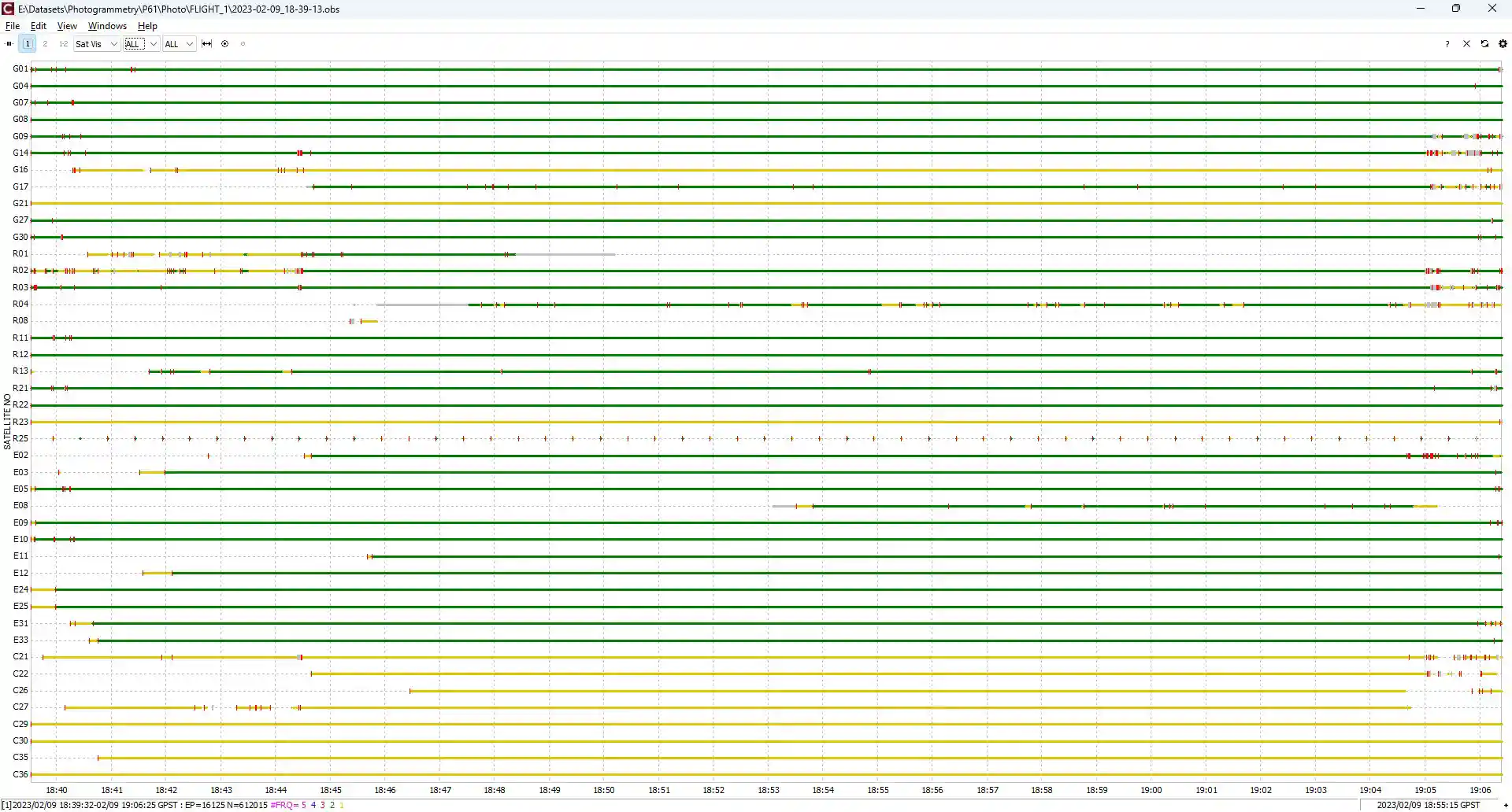
The Sat Vis (Satellite Visibility) window displays GNSS satellite visibility in dynamic graphical or tabular format, recording satellite availability for the receiver at specific time points.
Graph Structure:
-
X-axis: Time scale corresponding to the measurement session duration.
-
Y-axis: List of satellites with their respective navigation systems (e.g., G – GPS, R – GLONASS, E – Galileo, C – BeiDou).
-
Lines/bars: Represent periods when a satellite is visible to the receiver.
-
Color coding: Indicates GNSS signal frequency bands (e.g., yellow – L1, green – L1+L2, etc.).
Each bar corresponds to an individual satellite.
Bar length indicates satellite availability duration.
Gaps represent signal loss periods (e.g., due to obstructions).
Increasing the number of simultaneously tracked satellites can improve geometric diversity, reducing the DOP (Dilution of Precision) value. However, insufficient visible satellites may significantly degrade positioning accuracy.
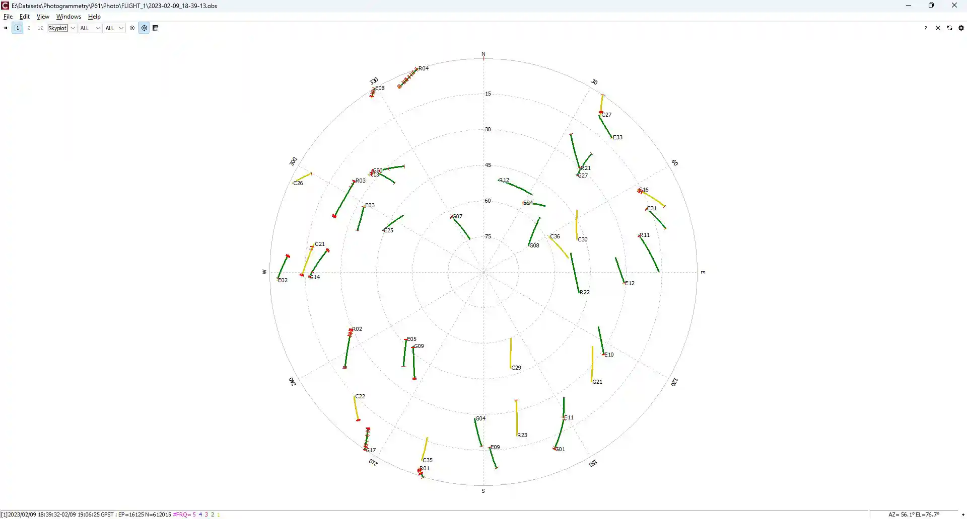
The Skyplot window visualizes GNSS satellite positions in a polar coordinate system, displaying their location in the celestial sphere relative to the receiver.
Diagram Structure:
The diagram is a circular "top-down" projection where:
-
Center represents the zenith (satellites directly above the receiver);
-
Outer circle denotes the horizon (satellites at minimum elevation angle);
-
Cardinal directions are standardized:
-
North (N) – top of the diagram,
-
East (E) – right side,
-
South (S) – bottom,
-
West (W) – left side.
-
The plot allows evaluation of:
-
Satellite distribution by azimuth and elevation angle;
-
Geometric diversity (critical for DOP calculation);
-
Potential signal obstruction zones (satellites near the horizon).
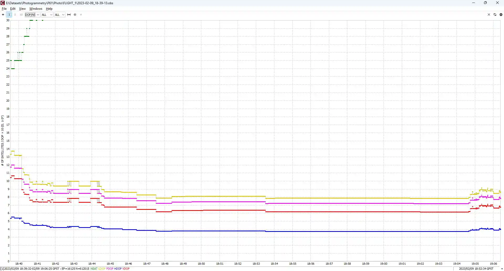
The DOP/NSat window provides key metrics for assessing GNSS positioning quality, reflecting both the spatial distribution of satellites and their quantity during measurements.
Key parameters:
-
DOP (Dilution Of Precision) - A coefficient quantifying the influence of satellite geometric configuration on positioning accuracy. The DOP value is determined by the relative positions of navigation satellites with respect to the receiver in three-dimensional space.
-
NSat (Number of Satellites) - A parameter indicating the number of satellites participating in the navigation solution at each time epoch.
DOP classification:
-
GDOP (Geometric DOP) - Comprehensive accuracy degradation metric for all components (3D coordinates + time offset)
-
PDOP (Position DOP) - Characterizes 3D positioning accuracy degradation (latitude, longitude, altitude)
-
HDOP (Horizontal DOP) - Reflects horizontal plane accuracy degradation (latitude, longitude)
-
VDOP (Vertical DOP) - Indicates height determination accuracy degradation. Under typical conditions, VDOP exceeds HDOP due to satellite constellation geometry specifics.
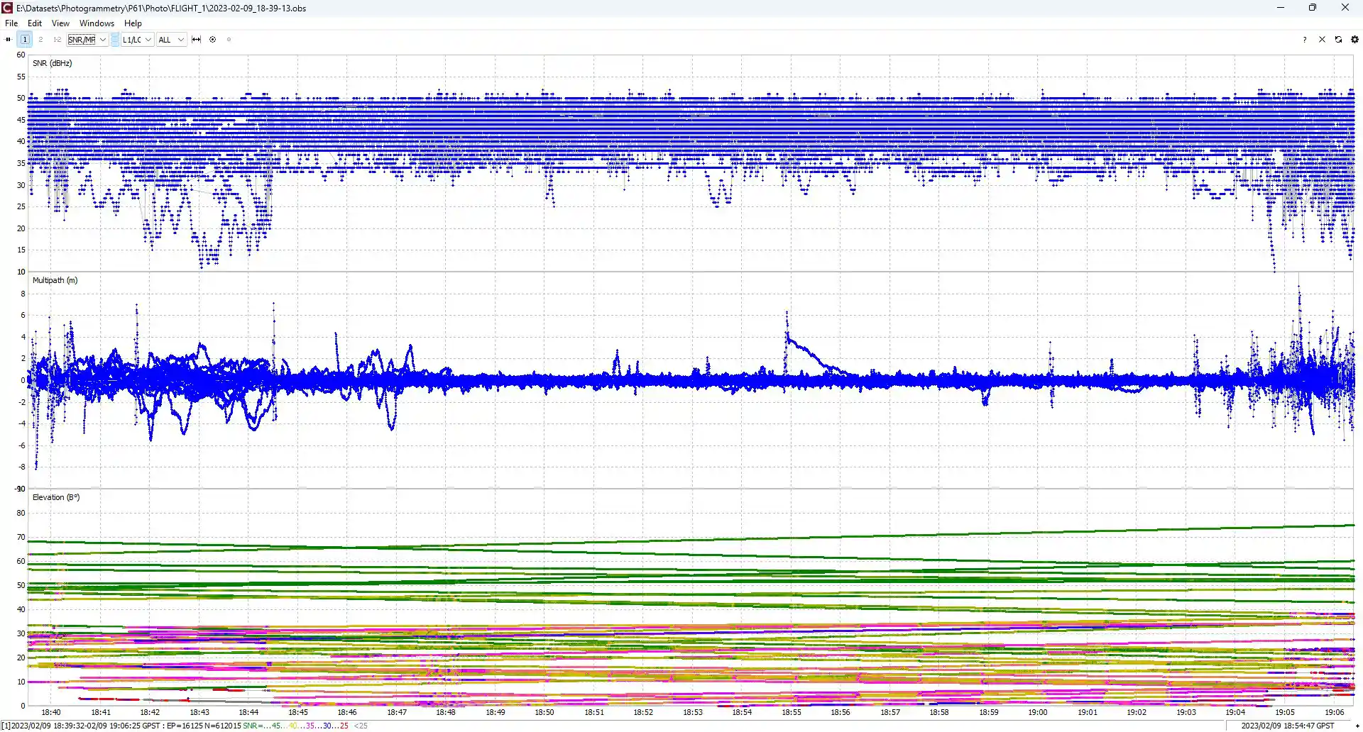
The SNR/MP/El window provides comprehensive diagnostics of key GNSS signal quality parameters. Let's examine the main parameters:
SNR (Signal-to-Noise Ratio) - The ratio of signal power to noise spectral density (dB-Hz).
-
Optimal values: >35 dB-Hz (high signal quality)
-
Critical values: <25 dB-Hz (risk of loss of lock)
MP (Multipath) - Phase distortions caused by multipath effects.
-
Evaluation scale:
- 0-0.5 m: negligible impact
- 0.5-1.0 m: moderate distortions
- 1 m: severe distortions due to reflected signals
El (Elevation Angle) - Satellite's vertical angle relative to local horizon (degrees).
-
Interpretation guidelines:
-
0°-15°: high noise and multipath zone
-
15°-30°: acceptable quality working zone
-
30° and above: optimal reception zone
-
Correlative parameter variations help identify:
Signal obstruction (simultaneous SNR and El drop)
Multipath effect (MP increase with stable SNR)
Atmospheric interference (sporadic SNR fluctuations)
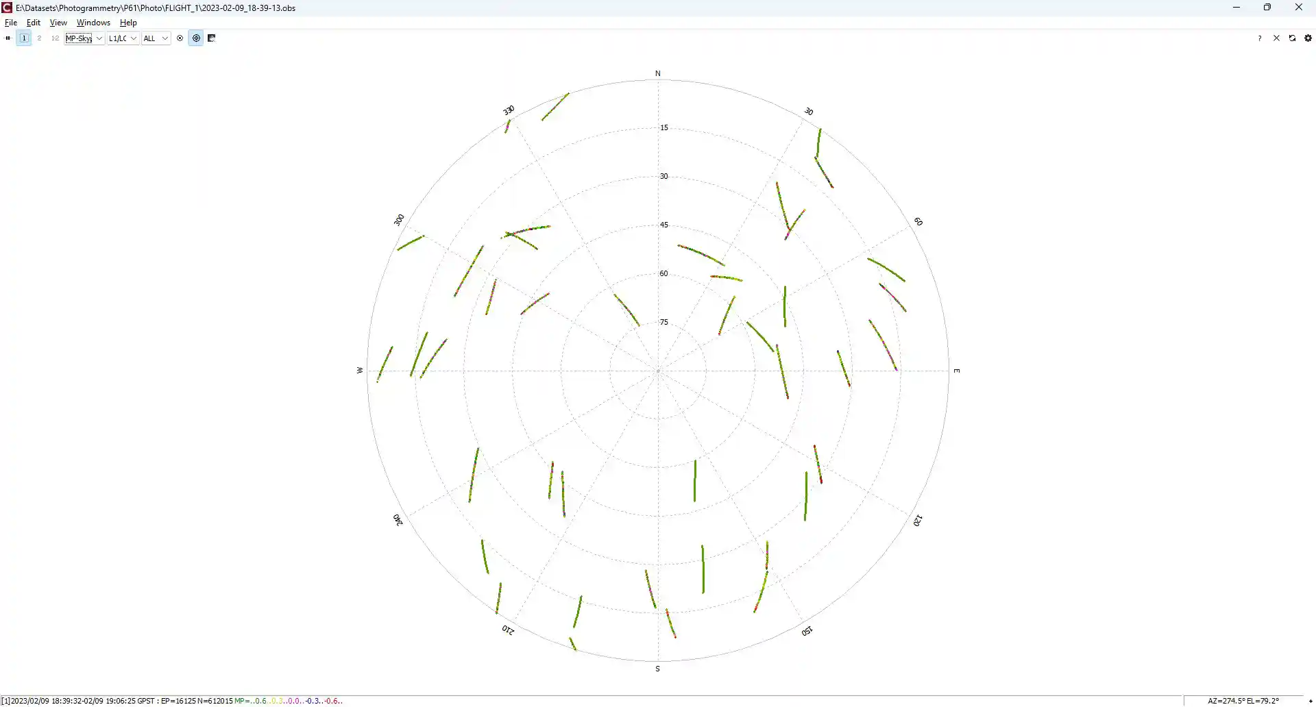
The MP-Skyplot window is a specialized visualization tool that combines multipath effect analysis with spatial satellite distribution in the celestial sphere.
This plot integrates:
-
Polar projection of satellite positions (similar to standard Skyplot)
-
Color/gradient indication of multipath distortion levels
Diagram structure features a circular top-down projection where:
-
Center represents the zenith (satellites directly above the receiver)
-
Circumference denotes the horizon (satellites at minimum elevation angle)
-
Cardinal directions follow standard orientation:
-
North (N) - top of diagram
-
East (E) - right side
-
South (S) - bottom
-
West (W) - left side
-
Release Notes
Software Operation Conditions After Technical Support Expiration
The operation of the TOPODRONE Post Processing distributor depends on the current technical support status. If the paid support period expires before the release date of a new software version, the user will not be able to use this distributor. The following options are available to continue working:
- Renewing technical support – activates access to the latest software versions.
- Using compatible distributors – installing versions released before the expiration date of the current active support.
The corresponding distributors are available for download at the following link: TOPODRONE Software Distributor
TPP v.1.5.3.0
November 11, 2025.
General Improvements
- Visualization.
- Fixed an error related to incorrect initialization of the takeoff point coordinates, which caused its default location to be set as the North Pole or a point with zero coordinates (0°, 0°).
- Performance.
- All calculations related to LiDAR point cloud processing are now performed in streaming mode, eliminating the limitation on the volume of loaded data.
PPK Post Processing
- Added support for a new modification of the Q.Fly Water SWIR camera for calculating the relative soil moisture and plant leaf moisture index.
New Utilities
- LAS/LAZ INSTA 360 Coloring
- A tool created for coloring point clouds from the Insta 360 camera during Mobile Laser Scanning (MLS) and for creating georeferenced panoramas.
- IMR Recovery.
- This tool allows calculating the trajectory of the laser scanner during short-term GNSS data losses.
TPP v.1.5.2.1
July 27, 2025.
General Improvements
- Licensing.
- Added display of the release date on the license information page.
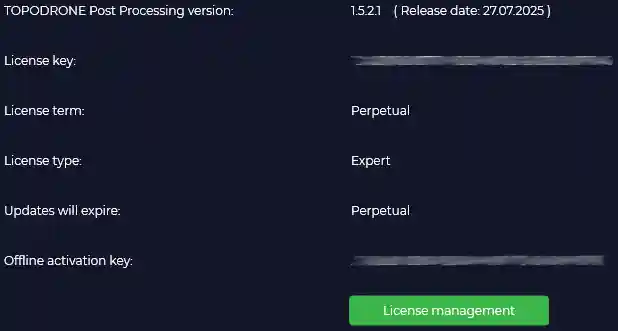
- Performance.
- Accelerated project (PRJ) loading at startup (optimization for ~6000 files);
- Improved data visualization speed (trajectories, photos, timestamps) across all modules.
- Data and Formats:
- Updated antenna file igs20_2353.atx;
- Integrated the lasinfo utility (LAStools) for checking LAS/LAZ headers;
- Added coordinate system information to LAS/LAZ headers;
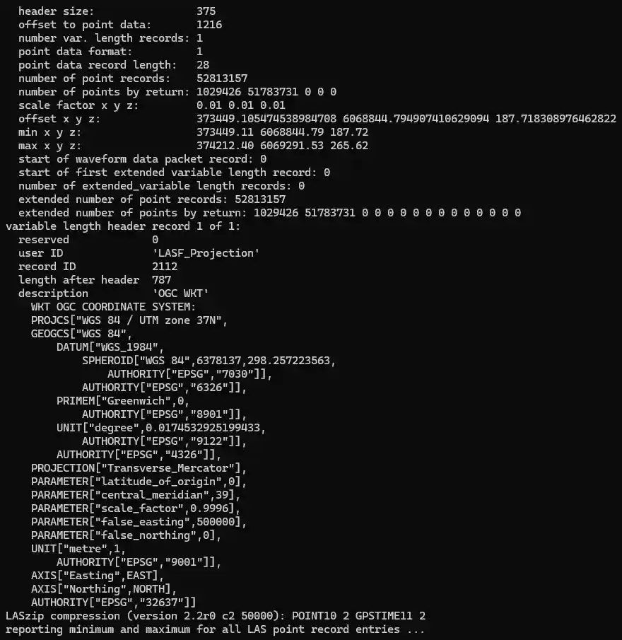
-
- Added the ability to convert point clouds (.LAS/.LAZ) between Coordinate Systems (in Tools).
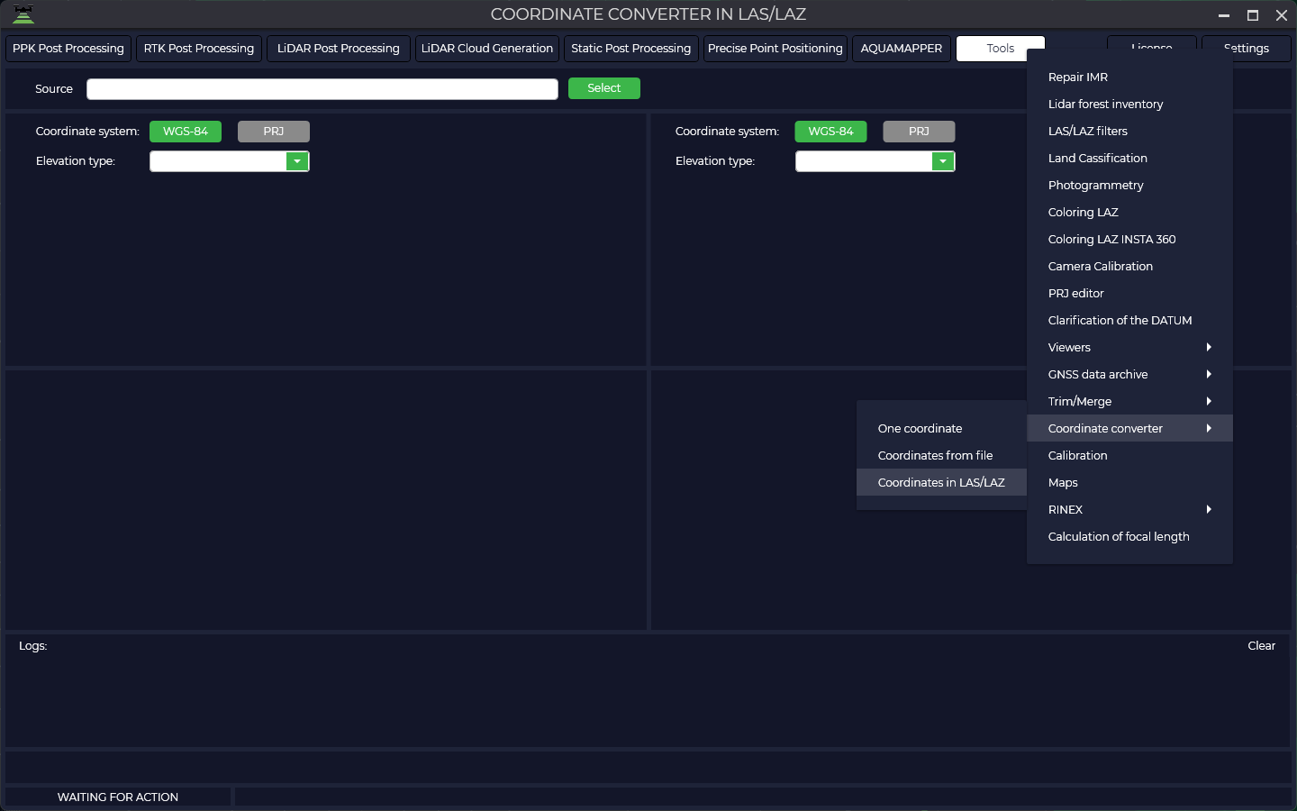
- GNSS Processing Settings:
- Added an option to disable GPS grouping when calculating trajectories;
- Removed frequency filtering (L1/L2...) – now all available frequencies are used.
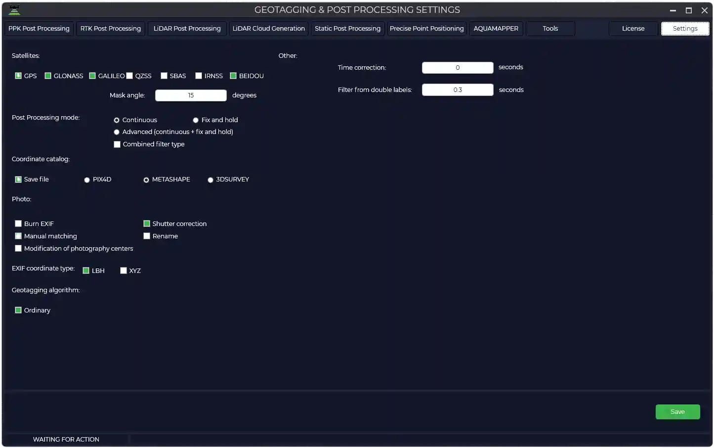
- Logging
- Processing journal maintained in logs.txt, including:
- Rover/base station activation time;
- Number of satellites;
- Used frequencies;
- Data recording rate and other parameters.
- Processing journal maintained in logs.txt, including:
25/07/2025 18:30:15
Dataset №1:
TPP Version: 1.5.2.1(27.07.2025)
License key: 1348DF06-8777-48CF-A6D8-E4239CA973A0
#Images folder: E:\Datasets\Photogrammetry\TOPODRONE P61 21 mm Orsha\Photo RGB
GNSS file: E:\Datasets\Photogrammetry\TOPODRONE P61 21 mm Orsha\Photo RGB\2023-07-05_11-01-12.ubx
Start time: 05/07/2023 11:01:31 UTC
End time:05/07/2023 11:26:52 UTC
Sampling Rate: 0.1 s (≈ 10 Hz)
Observed measurement types:
G (GPS): C1C D1C L1C S1C C2X D2X L2X S2X
R (GLONASS): C1C D1C L1C S1C C2C D2C L2C S2C
E (Galileo): C1X D1X L1X S1X C7X D7X L7X S7X
C (BeiDou): C2I D2I L2I S2I C7I D7I L7I S7I
Number of satellites observed:
Min: 29
Average: 40.6
Max: 42
Epochs : 15208 of 15208 expected ( 100.00% complete )
Number of photos: 304
Number of events: 304
Drone model: TOPODRONE P61+PPK+DJI Matrice 300
Forward/backward offset: 0.074
Left/Right offset: 0.022
Antenna height: 0.362
#Coordinate system: World-WGS 84-UTM-zone 35N (m) EPSG 32635
Geoid model: Ellipsoid WGS-84
#Base station: E:\Datasets\Photogrammetry\TOPODRONE P61 21 mm Orsha\ReachGeoGor_raw_20230705105548.obs
Start time: 05/07/2023 10:56:06 UTC
End time:05/07/2023 12:52:11 UTC
Sampling Rate: 1 s (≈ 1 Hz)
Observed measurement types:
G (GPS): C1C D1C L1C S1C C2X D2X L2X S2X
R (GLONASS): C1C D1C L1C S1C C2C D2C L2C S2C
E (Galileo): C1X D1X L1X S1X C7X D7X L7X S7X
S (SBAS): C1C D1C L1C S1C
C (BeiDou): C2I D2I L2I S2I C7I D7I L7I S7I
Number of satellites observed:
Min: 40
Average: 42.6
Max: 46
Epochs : 6966 of 6966 expected ( 100.00% complete )
North: 6045511.967295254
East: 701922.4288487637
Height: 228.738
Antenna height: 1.834
#Settings
Satellites: GPS GLONASS GALILEO BEIDOU
Mask angle: 15
Post Processing mode: Continuous / [ ] Combined filter type
Coordinate catalog: [x] Save file: Metashape
Photo: [ ] Burn EXIF
[x] Shutter correction
[x] Manual matching
[ ] Rename Photo
[ ] Modification of photography centers
EXIF coordinate type: [ ] LBH [x] XYZ
Geotagging algorithm: [x] Ordinary
[ ] Increase time weight
[ ] Increase weight of coordinates
Time correction: 0 seconds
Filter from double labels: 0.3 secondsPPK Post Processing
- Added support for the TOPODRONE Q.FLY camera.
RTK Post Processing
- Correction of the center of photography for DJI Matrice 4E by offsets from the MRK file;
- Added data processing with DJI Mavic 3 Multispectral.
LiDAR Cloud Generation
- Calculation of calibration angles has been significantly accelerated;
- New calibration algorithm for mobile laser scanning from a car — eliminates post-processing in third-party software.
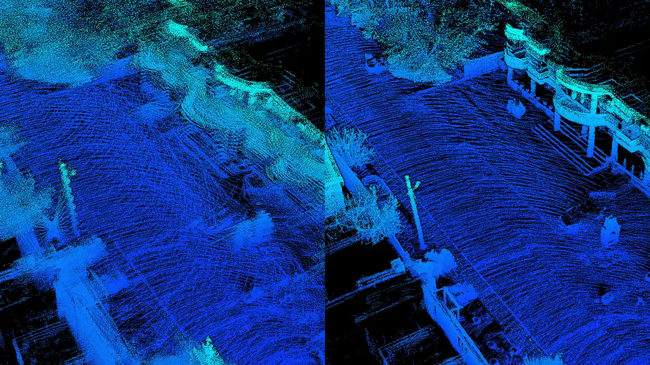
TPP v.1.5.1.4
March 07, 2025.
PPK Post Processing
- Added support for UNICORE GNSS chips for all TOPODRONE models.
- Added antenna offset presets for:
- TOPODRONE P24 New + PPK + DJI Matrice 350.
- Implemented automatic offset detection based on image tags.
- Antenna offset parameters are hidden from the interface (automatic calculation is used).
RTK Post Processing
- Implemented automatic loading of navigation files for each flight;
- Fixed the display of the "Plot" window in batch processing.
LiDAR Post Processing
- Fixed the display of the "Plot" window in batch processing.
LiDAR Cloud Generation
- Added generation of point clouds in local rectangular coordinates (in addition to global CS).
AQUMAPPER
- Automation:
- Added a filter to remove points with zero depth.
- Data Formats:
- Implemented separation of data from the dual-frequency TOPODRONE AQUAMAPPER Next sensor in .LAZ format:
- 200 kHz — 2nd return,
- 450 kHz — 1st return.
- Rounding values in .CSV (X/Y/Z coordinates, depths) to 3 decimal places.
- Implemented separation of data from the dual-frequency TOPODRONE AQUAMAPPER Next sensor in .LAZ format:
- Algorithms:
- Improved temperature calculation for each measurement (increased accuracy).
TPP v.1.5.1.3
January 25, 2025.
General Improvements
- Validation of base station and rover operation time.
- In the PPK Post Processing, RTK Post Processing, and LiDAR Post Processing modules, automatic validation of the correspondence between rover and base station data recording times has been implemented. A warning is displayed if the time intervals do not match: "Base station operation time does not match rover operation time." Standard processing is performed only with a complete match. For batch processing, the check is applied to all rover files.
- Checking for time gaps in IMU data.
- Added automatic checking of IMU measurement files for time gaps. If gaps are detected, a warning is displayed with the recommendation: "IMR file has time gaps, please use the 'IMR Trimming' tool."
- Interface Unification.
- Unified the sizes of the "Coordinate System", "Logs", and "Map" dialog windows in the specified modules.
RTK Post Processing
- Fixed an error where the "Plot" window (globe) call button was not displayed in the PPK Post Processing module, including batch processing mode.
TPP v.1.5.1.2
December 28, 2024.
General Improvements
- Launching the License Manager from the interface.
- Added a license information dialog with the ability to directly launch the "License Management Manager" from the TOPODRONE Post Processing interface.
- Updated the base RTKlib library (version j → k).
- Added a license information dialog with the ability to directly launch the "License Management Manager" from the TOPODRONE Post Processing interface.
PPK Post Processing
- Implemented automatic normalization of camera shutter release timestamps to a single format to eliminate the doubling effect. The new algorithm detects gaps in timestamps and adds missing data to the stream using an approximation method.
RTK Post Processing
- Adjustments have been made to the "Dynamic" function parameters. The update aims to reduce data processing errors during trajectory prediction. The new model accounts for the probability of sudden changes in the rover's dynamic parameters (speed and direction), allowing for more accurate position prediction under uncertainty.
LiDAR Cloud Generation
- Developed a new algorithm for calculating calibration angles by introducing a multiplier dependent on the speed of movement, which accelerates the time to find corrections.
AQUMAPPER
- Added support for a dual-frequency echosounder (200 kHz + 450 kHz). The low-frequency signal (200 kHz) provides greater penetration depth, while the high-frequency signal (450 kHz) provides higher clarity and detail of the bottom. The combined use of frequencies increases both the survey depth and the ability to separate weak signals for detailed data.
- Added trajectory display in the "Plot" window.
TPP v.1.4.5.0
November 12, 2024.
PPK Post Processing
- Implemented support for UNICORE GNSS receivers.
- Improved the algorithm for generating georeferencing files used for coloring point clouds obtained from TOPODRONE laser scanners.
RTK Post Processing
- Ensured correct conversion of files from
.binto.obsand.navformats.
TPP v.1.4.4.4
November 04, 2024.
PPK Post Processing
- Added automatic creation of a camera shutter event timestamp file for subsequent use in the point cloud coloring utility for point clouds obtained by TOPODRONE laser scanners.
RTK Post Processing
- Ensured correct conversion of data from the proprietary
.binformat to the standard RINEX format.
LiDAR Post Processing
- Before sending for processing on the server, the base station measurement file in *.**O format is automatically converted to *obs format to ensure compatibility.
New Utilities
- Distortion Correction.
- Implemented a new camera calibration utility designed to calculate interior orientation parameters: principal point coordinates, focal length, radial and tangential distortion coefficients on photographs.
- Point Cloud Texturing.
- Added a utility for coloring point clouds using photo data when using a photogrammetric camera and a TOPODRONE laser scanner together.
TPP v.1.4.4.2
October 02, 2024.
General Improvements
- Added a "Clear Logs" button in all modules for quick clearing of the processing log window.
- Coordinate system files (*.prj) are now stored on the server. Added a function to download them via the "General Settings" section.
PPK Post Processing / RTK Post Processing
- Updated and fixed configuration files for the modules.
LiDAR Cloud Generation
- Optimized the calibration angle calculation algorithm. The number of iterative passes is limited to 10 to prevent excessive computations.
Static Post Processing / PPP
- Updated sources for automatic ephemeris download. Now using University of California, San Diego (UCSD) servers instead of NASA to ensure data availability for every day.
AQUAMAPPER
- Ensured correct data processing when GNSS equipment time crosses midnight and during batch calculation of datasets collected over several weeks.
TPP v.1.4.4.1
September 10, 2024.
PPK Post Processing / RTK Post Processing
- Speed data in output files is now correctly read from
event.pos. Previously, thepos.statfile was erroneously used, which in some scenarios contained zero values. - Eliminated unwanted reset of the map view to coordinates (0;0) after processing trajectories for cameras without navigation data. The map view now remains unchanged.
- Fixed an error where after processing data from the TOPODRONE PT61 camera, previews for a non-existent thermal sensor were erroneously generated for other cameras.
LiDAR Post Processing
- Implemented the ability to enter base station coordinates directly in a local coordinate system, considering the geoid model.
LiDAR Cloud Generation
- When generating multiple clouds from a single trajectory, each copy of the trajectory in the LCS (Local Coordinate System) receives a unique prefix
_HHMMSS(hours-minutes-seconds of generation), preventing them from being overwritten. - The algorithm for finding calibration angles has been supplemented with automatic calculation of a heading scaling factor depending on the speed of movement, significantly reducing the required number of iterative passes.
AQUAMAPPER
- Added the ability to simultaneously load and process data in UBX format during batch processing.
Utilities
- In the "IMR File Viewer" utility, the vibration graph is now displayed with a baseline "set to 0" for more visual analysis.
- The parsing algorithm for data from Livox MID-360 sensors has been refined, ensuring their complete and accurate processing.
TPP v.1.4.4.0
August 13, 2024.
PPK Post Processing
- Fixed incorrect preview image generation for the thermal imager of the TOODRONE PT61 camera. The algorithm now correctly processes sensors of different sizes (320 and 640 pixels).
- Fixed an error where a different number of photos from the TOPODRONE PT61 camera and timestamps led to the skipping of the manual matching window and, consequently, the absence of an output photo center catalog.
PPK Post Processing / RTK Post Processing
- Ensured correct column formation and file structure when exporting the photo center catalog for Agisoft Metashape and 3DSurvey software.
- The "Timestamp Correction" field has been returned to the photogrammetry parameters in the settings.
Tools
- Datum Parameters Calculation.
- Implemented a proprietary algorithm for calculating datum parameters for coordinate systems. Previously, a third-party library was used; now, a proprietary solution is applied for improved accuracy and transformation control.
- Merge track files.
- Fixed incorrect header formation when performing the track mergeing operation.
- Calibration.
- Added an "Open Catalog" button to the calibration interface for loading point catalogs.
- Ground Classification
- Added an option – "Slope Processing" to the ground classification module to improve terrain analysis.
- IMR Viewer
- Added display of vibration graphs along the axes to the utility for detailed analysis of inertial system data quality.
TPP v.1.4.3.0
July 30, 2024.
AQUAMAPPER
- Data processing settings have been moved to the user interface (UI) for more convenient and flexible parameter management.
- Added infographics displaying key parameters: equipment roll, pitch, and bottom topography for surveying data quality control.
Tools
- Added a new utility «3DFine: Forest Inventory»
- The utility is designed for automated analysis of laser scanning data for the purpose of forest taxation. The utility's algorithms automatically detect trees, calculate taxation indicators such as height, Diameter at Breast Height (DBH), and cross-sectional area, and generate standard reports for forestry.
TPP v.1.4.2.0
June 20, 2024.
PPK Post Processing
- Added support for the TOPODRONE PT61 camera, including with AGROWING multispectral lenses.
Tools
- Point Cloud Viewer. Updated PotreeConverter from version 1.7 to 2.1.
TPP v.1.3.3.4
April 23, 2024.
Tools
- Trim IMR. Added the ability to trim a file obtained from an inertial sensor without loading data from a geodetic receiver.
TPP v.1.3.3.0
April 05, 2024.
LiDAR Post Processing
- During batch calculation of high-precision tracks, 10 times fewer points are displayed on the map for visualization to optimize performance. This solves the problem of the program interface "freezing" when rendering tracks containing a large number of points.
LiDAR Cloud Generation
- Implemented a new, improved algorithm for calculating scanner installation calibration angles, providing increased accuracy and stability of results.
- Fixed: The function for trimming beam length for data from laser scanners with Hesai sensors now works correctly.
- SLAM Processing. To improve registration accuracy, returning the point cloud to the track is performed using calibration parameters.
TPP v.1.3.2.2
March 17, 2024.
General Improvements
- Automatic Dependency Installation.
- Key dependencies (WinPcap and .NET Core 3.1 Desktop Runtime) are now installed automatically during the distributor installation process, relieving the user from the need for manual environment setup.
LiDAR Cloud Generation
- Implemented a new iterative algorithm for calculating calibration angles. Angles are calculated and applied stepwise for gradual refinement and correction of track tilt, significantly improving the accuracy of the final point cloud.
AQUAMAPPER
- The AQUAMAPPER module for comprehensive processing of hydrographic survey data has been fully integrated into the distributor.
TPP v.1.2.0.1
November 23, 2023.
LiDAR Post Processing
- Implemented switching between Standard and Expert operation modes in the program settings.
- Standard Mode: Performs automatic detection of IMU and LiDAR models, simplifying setup for the user.
- Expert Mode: Provides the ability to manually select specific IMU and LiDAR models from a list for full control over processing parameters.
TPP v.1.2.0.0
November 20, 2023.
LiDAR Post Processing
- Implemented an alternative algorithm for calculating track coordinates based on comprehensive processing of information from the angular navigation hardware platform and GNSS.
LiDAR Cloud Generation
- Survey type (Aerial / Terrestrial) is determined automatically based on the processed trajectory.
- The position of the laser scanner sensor (Forward / Backward) is determined automatically based on the processed trajectory, eliminating errors from manual assignment.
TPP v.1.1.17.0
November 13, 2023.
LiDAR Cloud Generation
- Implemented an algorithm for automatic detection and application of UTM (Universal Transverse Mercator) projection based on the point cloud center coordinates, if the user did not explicitly specify a coordinate system in the settings.
Static Post Processing
- Implemented a function for automatic reading and adding of navigation coordinates from the headers of base station GNSS files. This simplifies the initial processing setup, especially when working with a large number of sessions.
TPP v.1.1.16.1
November 01, 2023.
PPK Post Post Processing / RTK Post Processing / Static Post Processing / Precise Point Positioning
- The combined Kalman filter is now enabled by default. Using this filter significantly improves the accuracy and smoothness of the calculated trajectories.
TPP v.1.1.16.0
October 30, 2023.
LiDAR Cloud Generation
- Implemented a new algorithm for finding calibration angles based on ICP (Iterative Closest Point). This method uses iterative point cloud matching for accurate calculation of LiDAR installation angles, significantly improving calibration accuracy.
- Added support for the Livox MID-360 LiDAR, including automatic recognition, data parsing, and calculation of calibration parameters.
TPP v.1.1.15.0
October 04, 2023.
PPK Post Processing / RTK Post Processing
- Completely updated the built-in catalog of GNSS antenna models. Updated antenna parameters improve phase center offset corrections and, consequently, overall GNSS processing accuracy.
Tools
- Added a new utility «Datum Refinement». The tool allows performing high-precision transformation and calculation of transition parameters between coordinate systems based on point catalogs.
TPP v.1.1.14.0
September 20, 2023.
LiDAR Post Processing Settings
- Added the ability to specify LiDAR rotation relative to the IMU (roll/pitch/heading).
New Utilities
- PRJ Editor
- The utility allows correcting PRJ file parameters.
TPP v.1.1.13.0
August 29, 2023.
General Improvements
- Added automated download of geoids from the TOPODRONE server (199 geoids). Geoids are no longer included in the distributor (reducing distributor size) and are downloaded by users as needed.
New Modules
- Photogrammetry
- Added a module for photogrammetric processing
TPP v.1.1.12.0
August 22, 2023.
General Improvements
- Integrated a new version of the high-precision trajectory calculation algorithm with support for current TOPODRONE equipment.
- Updated the LAS/LAZ processing library (support for formats 1.3/1.4).
Laser Scanning Data Processing
- Added filters to improve the quality of the laser scanning point cloud: SOR and NOISE.
New Utilities
- Ground Classification
- Added a utility that allows performing automatic terrain classification.
TPP v.1.1.11.1
August 08, 2023.
LiDAR Cloud Generation Settings
- For Hesai sensors, implemented an offset of the emitter's optical axis relative to the geometric center of the sensor's sensitive area.
TPP v.1.1.9.1
June 24, 2023.
PPK Post Processing / RTK Post Processing / LiDAR Cloud Generation
- Implemented a new coordinate system filtering system using progressive full-text search. Results are displayed as a list where each item represents the full projection name.
TPP v.1.1.9.0
June 04, 2023.
General Improvements
- The satellite filtering utility has been accelerated by 50 times.
- A "ruler" for distance measurements has been added to all maps. Double-click on the map and the distance between these points will be written in the logs (in feet or meters depending on the state of the "Feet" checkbox).
New Algorithms
- TOPOSLAM
- Added a new algorithm consisting of three stages. The first stage performs sequential cloud alignment by generation time. The second stage performs mutual alignment of the nearest clouds by distance. The third stage, using calibration, returns the position of the aligned clouds to the track.