
Grid equalization
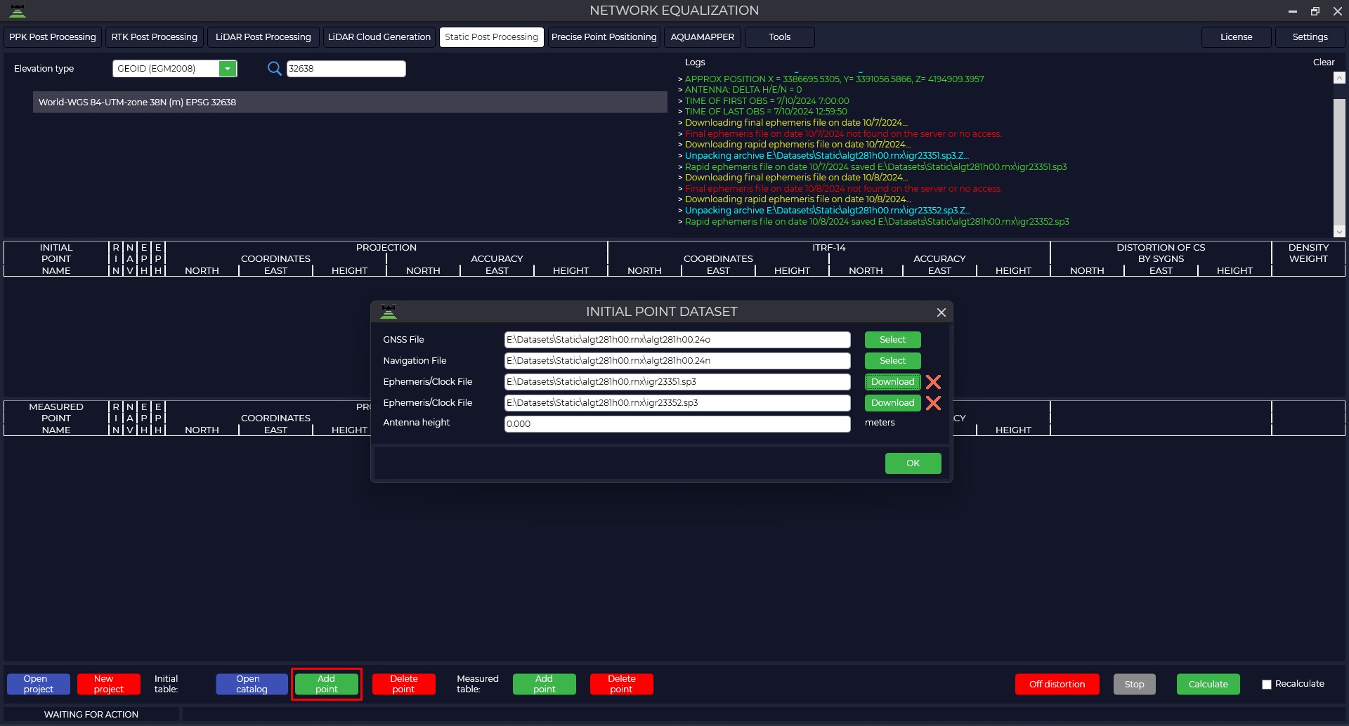
- To start this module, go to the Static Post Processing tab and click on the Network Equalization button.
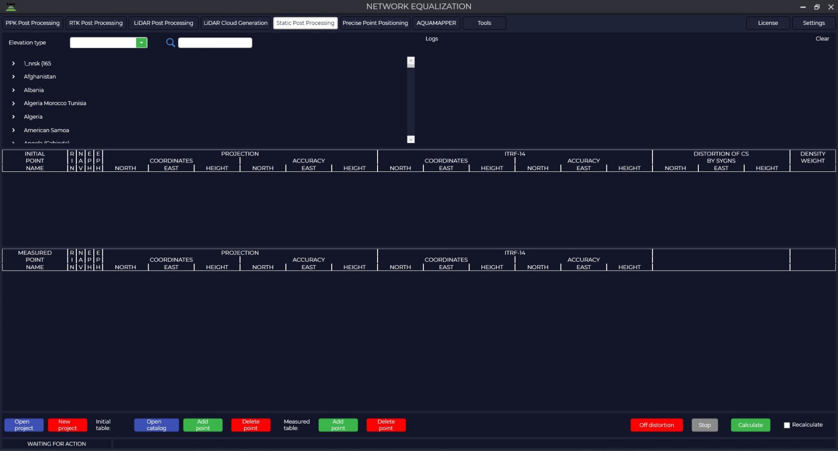
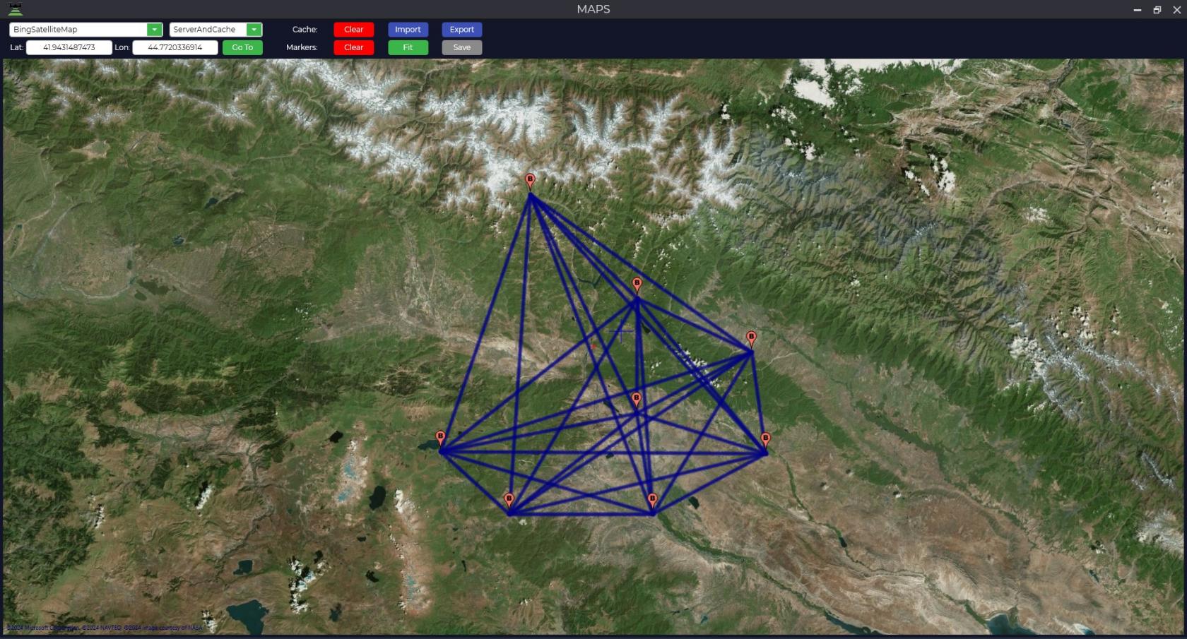
- To display the points where observations were made, the map window must be open at the time of file upload.
- The bottom panel has a number of tools: open or create a new project, open the source point catalog, add or delete source point files, add or delete measured point files, remove projection distortions, stop processing, and calculate.

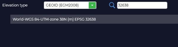
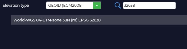
- The first thing to do is to select the required projection and the type of elevation to be used.
- When we click on the "Add Point" button next to the "Start Table" item, we need to load the data for the starting points.

GNSS file - a GNSS receiver measurement file in *.obs, *.rnx or *.*o formats.
Navigation file - navigation file of measurements in *.nav, *.rnx, *.n, *.p, *.g, *.h, *.q, *.c and *.l format.
Ephemeris file - file of final ephemeris in *.sp3, *.eph format, you can also upload a file of accurate flight clock *.clk. When you click on the Download button, if the data are available on the NASA server, the program will automatically download these data.
When processing the Grid Equation, the program uses the method of obtaining Precise Point Positioning (PPP) coordinates of the terrain using global navigation satellite systems by obtaining corrections to the orbital ephemeris and on-board clocks of all visible spacecraft. For the best calculation it is recommended to add daily measurements from the nearest reference base station or IGS.
Antenna height is the height from the center of the point to the phase center of the GNSS receiver.
Type Accuracy of orbits and clocks Accessibility Note Broadcast ~100 см
~5 ns RMS
~2.5 ns σIn real time GLONASS (.YYg) and GPS (.YYn) on-board ephemeris for a day in RINEX format summarized in the TsUP UltraRapid ~3 см
~150 ns RMS
~50 ns σIn 3-9 hours Refined ephemeris and corrections of airborne clocks Rapid ~2.5 см
~75 ns RMS
~25 ns σAfter 17-41 hours Ephemeris and corrections of onboard clocks obtained on the interval of last days Final ~2.5 см
~75 ns RMS
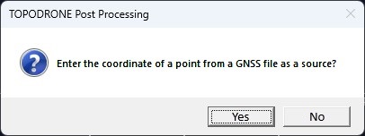
~20 ns σAfter 12-18 days Final ephemeris and flight clock corrections - When adding initial data to the program, a window will appear on entering coordinates of the point from the loaded file, click the "Yes" button.
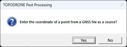
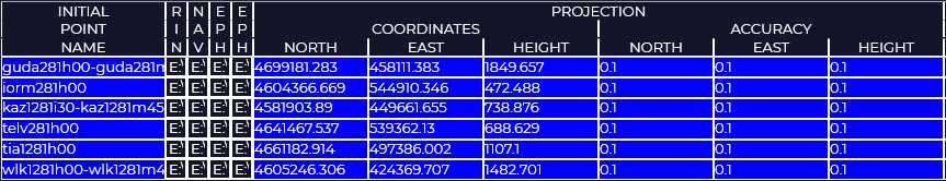
- Then, if necessary, load the coordinate catalog of the source points or enter the coordinates and their accuracy manually.

If you do not know with what accuracy they have been determined, you should provide the following recommended accuracies:
• FAGS 20 mm north/east, 30 mm high;
• HCV 30mm north/east, 40mm high;
• AGS and GHS 40mm north/east, 50mm high;
• GGS 60mm north/east, 110mm high.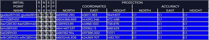
- To load the data for measured points, you must use "Add point" against the item "Measurement table" and perform the loading by analogy with the original points.

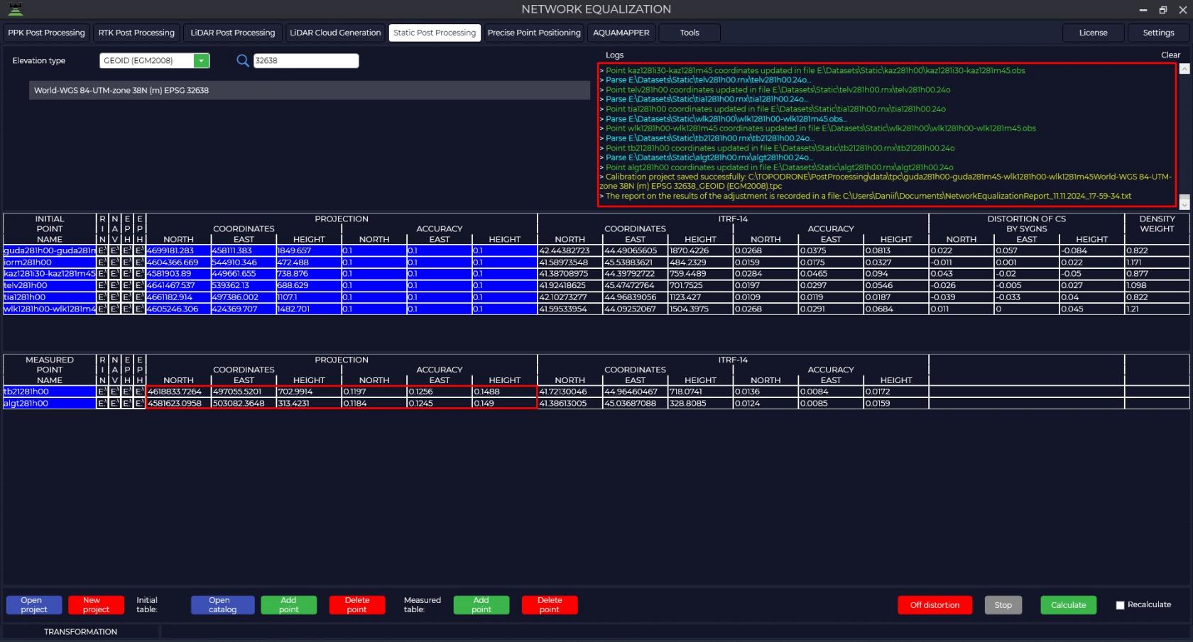
- Once all items have been loaded, click on the "Start" button and the program will begin the calculation. The number of operations and the total number of calculations to be performed will be displayed on the bottom left.
The calculation of the network follows the following algorithm: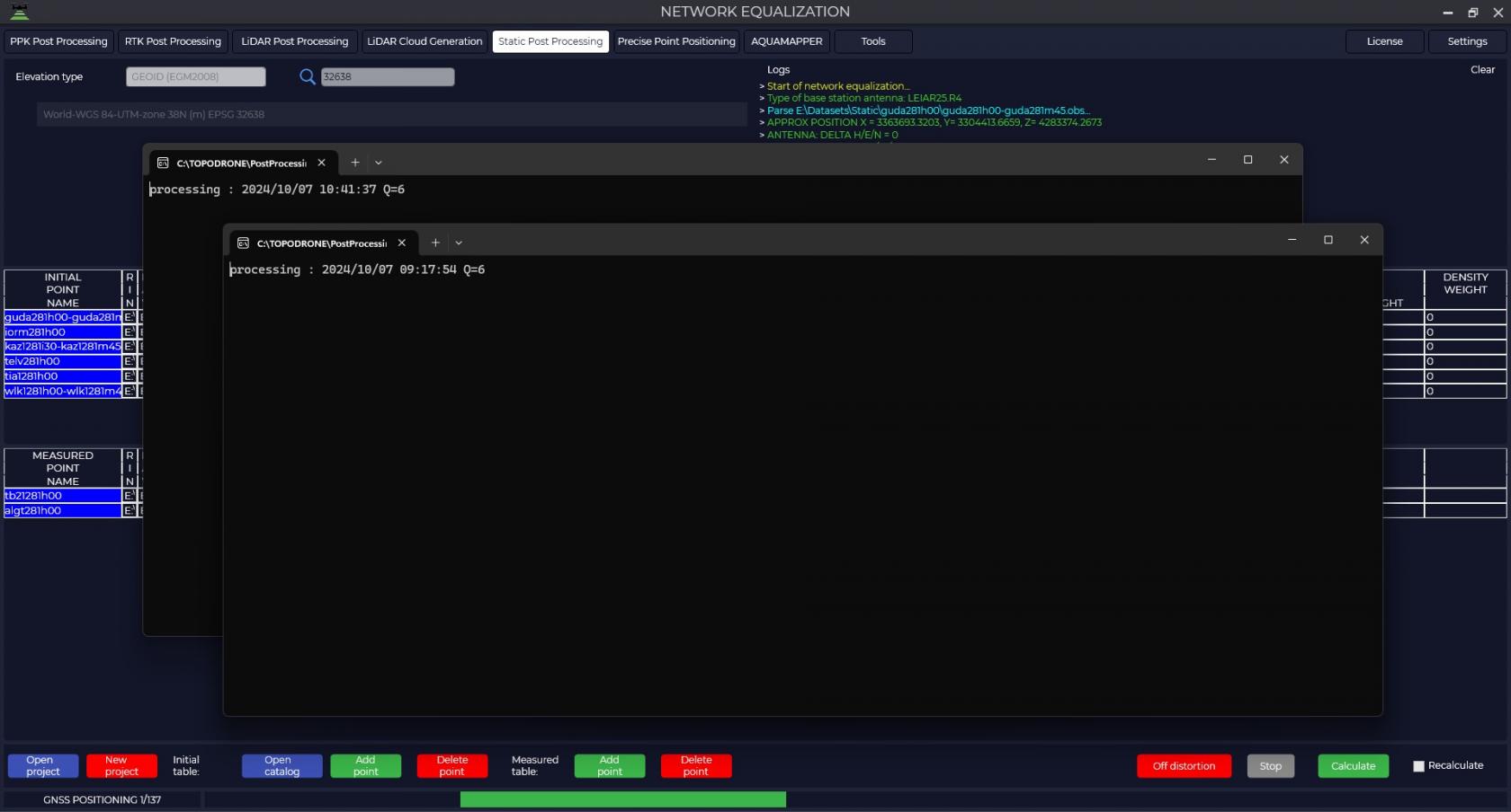
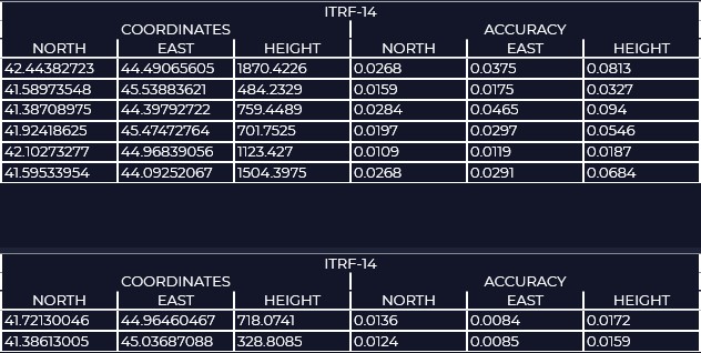
1) Calculation of coordinates of all points in ITRF2014 coordinate system by Precise Point Positioning - PPP method. After this step in the ITRF-14 window you will see the calculated coordinates and their accuracy.
2) In the next step, the program performs Precise Point Positioning and static measurement of all possible vectors, performs point coordinates calculation by precision weighting.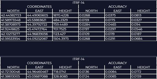
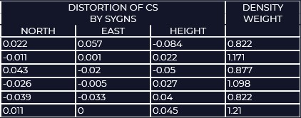
3) Then, using the coordinate system and coordinates of the initial points, taking into account the weighting accuracies of the points, the program calculates the total displacement from the parameters of the selected projection and creates a grid of residual distortion corrections. - In the DISTORTION OF CS BY SYGNS window you can see the residual distortions of the coordinate system relative to the original points. In the DENSITY WEIGHT window Density of points, it is needed to increase/decrease the weight of distortions, a single point has a higher weight than a point that is next to others.
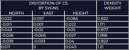
-
As a result of calculations you will get a catalog of coordinates of points in the coordinate system that was specified, accuracy of determination of these coordinates and distortion grid for use in the TOPODRONE Post Processing program. The calibration file can be opened through the "Tools" module, "Calibration" tab. In addition, a report of the processing results will be saved in the document folder.
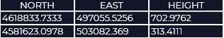
- When you click the "Correct Distortion" button, the program distributes the errors to the source items and re-runs the processing.

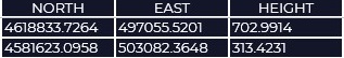
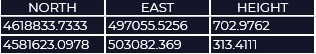
- The table below summarizes the results of processing
Caption Until distortion is eliminated After removing distortion 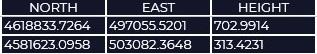


No Comments